Example C-level Portfolio

My Grade: I believe my grade equivalent to course work evidenced below to be an _A_.

Learning Objective Evidence: In the code chunks below, provide code from Lab or Challenge assignments where you believe you have demonstrated proficiency with the specified learning target. Be sure to specify where the code came from (e.g., Lab 4 Question 2).

Working with Data

WD-1: I can import data from a variety of formats (e.g., csv, xlsx, txt, etc.).

• csv

# Lab 2 Question  1

surveys <- read_csv(here::here("data", "surveys.csv"))

• xlsx

# Check-in 2.3 question 5

agesxl <- read_xlsx(path = here::here("check-ins", "2.1-loading-data", "Ages_Data", "ages.xlsx"), 
                    sheet = "ages")

• txt

# Checkins 2.3 question 4

ages_mystery <- read_delim(file = here::here("Week2", "Check-ins", "Ages_Data", "ages_mystery.txt"), delim="|")

WD-2: I can select necessary columns from a dataset.

# Lab 3 question 4

teacher_evals_clean <- teacher_evals |> 
  rename(sex = gender) |>
  filter(no_participants > 10) |> 
  mutate(
    across(.cols = c(teacher_id:class_duration), as.numeric)
  ) |> 
  select(course_id:SET_score_avg, percent_failed, academic_degree, seniority, sex)

WD-3: I can filter rows from a dataframe for a variety of data types (e.g., numeric, integer, character, factor, date).

• numeric

# Lab 3 question 9

teacher_evals_clean |> 
  count(course_id, teacher_id) |>
  filter(n == 9) |>
  nrow()

• character – specifically a string (example must use functions from stringr)

# PA-5 question 6

tibble(message) |>
  mutate(string_length = str_length(message)) |>
  slice_max(order_by = string_length,
            n = 1) |>
  select(message)

• factor

# Lab 4 question 6
ca_childcare |> 
  pivot_longer(cols = mc_infant:mc_preschool,
               names_to = "study_group",
               values_to = "median_amount") |>
  select(study_year, study_group, median_amount, region) |>
  mutate(study_group = str_to_title(str_remove(study_group, "mc_")),
         study_group = fct_relevel(study_group, "Infant", "Toddler", "Preschool")) |>
  ggplot(mapping = aes(x = study_year,
                       y = median_amount,
                       color = fct_reorder2(region, study_year, median_amount))) + 
  geom_point() +
  facet_wrap(~study_group) +
  geom_smooth(method = "loess") +
  labs(
    x = "Study Year",
    y = "",
    title = "Weekly Median Price for Center-Based Childcare ($)",
    color = "California Region"
  ) +
  theme_bw()

• date (example must use functions from lubridate)

# Lab 5

sql_city_crimes <- crime_scene_report |>
  filter(
    city == "SQL City",
    ymd(date) == ymd("20180115")
  )

WD-4: I can modify existing variables and create new variables in a dataframe for a variety of data types (e.g., numeric, integer, character, factor, date).

• numeric (using as.numeric() is not sufficient)

# Lab 3 question 4

teacher_evals_clean <- teacher_evals |> 
  rename(sex = gender) |>
  filter(no_participants > 10) |> 
  mutate(
    across(.cols = c(teacher_id:class_duration), as.numeric)
  ) |> 
  select(course_id:SET_score_avg, percent_failed, academic_degree, seniority, sex)

• character – specifically a string (example must use functions from stringr)

# Lab 4 question 3

ca_childcare <- ca_childcare |> 
  mutate(county_name = str_remove(county_name, " County")) |>
  mutate(region = fct_collapse(county_name,
                              "Superior California" = c("Butte", "Colusa", "El Dorado", "Glenn", "Lassen", "Modoc", "Nevada", "Placer", "Plumas", "Sacramento", "Shasta", "Sierra", "Siskiyou", "Sutter", "Tehama","Yolo", "Yuba"),
                              "North Coast" = c("Del Norte", "Humboldt", "Lake", "Mendocino", "Napa", "Sonoma", "Trinity"),
                              "San Francisco Bay Area" = c("Alameda", "Contra Costa", "Marin", "San Francisco", "San Mateo",
             "Santa Clara", "Solano"),
                              "Northern San Joaquin Valley" = c("Alpine", "Amador", "Calaveras", "Madera", "Mariposa", "Merced", "Mono",
             "San Joaquin", "Stanislaus", "Tuolumne"),
                              "Central Coast" = c("Monterey", "San Benito", "San Luis Obispo", "Santa Barbara", "Santa Cruz","Ventura"),
                              "Southern San Joaquin Valley" = c("Fresno", "Inyo", "Kern", "Kings", "Tulare"),
                              "Inland Empire" = c("Riverside", "San Bernardino"),
                              "Los Angeles County" = c("Los Angeles"),
                              "Orange County" = c("Orange"),
                              "San Diego-Imperial" = c("Imperial", "San Diego")
  ))

• factor (example must use functions from forcats)

# Lab 4 question 3

ca_childcare <- ca_childcare |> 
  mutate(county_name = str_remove(county_name, " County")) |>
  mutate(region = fct_collapse(county_name,
                              "Superior California" = c("Butte", "Colusa", "El Dorado", "Glenn", "Lassen", "Modoc", "Nevada", "Placer", "Plumas", "Sacramento", "Shasta", "Sierra", "Siskiyou", "Sutter", "Tehama","Yolo", "Yuba"),
                              "North Coast" = c("Del Norte", "Humboldt", "Lake", "Mendocino", "Napa", "Sonoma", "Trinity"),
                              "San Francisco Bay Area" = c("Alameda", "Contra Costa", "Marin", "San Francisco", "San Mateo",
             "Santa Clara", "Solano"),
                              "Northern San Joaquin Valley" = c("Alpine", "Amador", "Calaveras", "Madera", "Mariposa", "Merced", "Mono",
             "San Joaquin", "Stanislaus", "Tuolumne"),
                              "Central Coast" = c("Monterey", "San Benito", "San Luis Obispo", "Santa Barbara", "Santa Cruz","Ventura"),
                              "Southern San Joaquin Valley" = c("Fresno", "Inyo", "Kern", "Kings", "Tulare"),
                              "Inland Empire" = c("Riverside", "San Bernardino"),
                              "Los Angeles County" = c("Los Angeles"),
                              "Orange County" = c("Orange"),
                              "San Diego County" = c("Imperial", "San Diego")
  ))

• date (example must use functions from lubridate)

# Lab 5
sql_city_crimes <- crime_scene_report |>
  filter(
    city == "SQL City",
    ymd(date) == ymd("20180115")
  )

WD-5: I can use mutating joins to combine multiple dataframes.

• left_join()

• right_join()

• inner_join()

# Lab 5
witness_1_interview <- person |>
  filter(address_street_name == "Northwestern Dr") |>
  slice_max(order_by = address_number, n = 1) |>
  inner_join(interview, join_by(id == person_id))

WD-6: I can use filtering joins to filter rows from a dataframe.

• semi_join()

• anti_join()

WD-7: I can pivot dataframes from long to wide and visa versa

• pivot_longer()

# Lab 4 question 6

ca_childcare |> 
  # data cleaning
  pivot_longer(cols = mc_infant:mc_preschool,
               names_to = "study_group",
               values_to = "median_amount") |>
  select(study_year, study_group, median_amount, region) |>
  mutate(study_group = str_to_title(str_remove(study_group, "mc_")),
         study_group = fct_relevel(study_group, "Infant", "Toddler", "Preschool")) |>
  # plot
  ggplot(mapping = aes(x = study_year,
                       y = median_amount,
                       color = fct_reorder2(region, study_year, median_amount))) + 
  geom_point() +
  facet_wrap(~study_group) +
  geom_smooth(method = "loess") +
  labs(
    x = "Study Year",
    y = "",
    subtitle = "Weekly Median Price for Center-Based Childcare ($)",
    color = "California Region"
  ) +
  scale_x_continuous(breaks = seq(2008,
                                  2018,
                                  by = 2)) +
  theme_bw() +
  theme(
    aspect.ratio = 1.0,
    axis.text = element_text(size = 6)
  )

• pivot_wider()

# lab 4 question 4

ca_childcare |>
  filter(study_year %in% c(2008, 2018)) |>
  group_by(study_year, region) |>
  summarize(median = median(mhi_2018)) |>
  pivot_wider(id_cols = region,
              names_from = study_year,
              values_from = median)

Reproducibility

R-1: I can create professional looking, reproducible analyses using RStudio projects, Quarto documents, and the here package.

I’ve done this in the following provided assignments:

R-2: I can write well documented and tidy code.

• Example of ggplot2 plotting

# Lab 2 question 4
ggplot(data = surveys, aes(x = weight, y = hindfoot_length)) +
  geom_point(alpha = 0.5) +
  facet_wrap(~species) +
  labs(
    title = "relationship between weight and hindfoot_length of different species",
    subtitle = "y-axis representing hindfoot_length (mm)",
    x = "weight (g)",  # x-axis label
    y = ""
  )

• Example of dplyr pipeline

# Lab 3 question 11
teacher_evals_clean |>
  filter(seniority == 1) |>
  group_by(teacher_id) |>
  summarize(average_student_failing = mean(percent_failed)) |>
  filter(average_student_failing >= max(average_student_failing) | average_student_failing <= min(average_student_failing)) |>
  select(teacher_id, average_student_failing)

• Example of function formatting

R-3: I can write robust programs that are resistant to changes in inputs.

• Example – any context

# Lab 3 quetsion 5
teacher_evals_clean <- teacher_evals |> 
  rename(sex = gender) |>
  filter(no_participants > 10) |> 
  mutate(
    across(.cols = c(teacher_id:class_duration), as.numeric)
  ) |> 
  select(course_id:SET_score_avg, percent_failed, academic_degree, seniority, sex)

• Example of function stops

Data Visualization & Summarization

DVS-1: I can create visualizations for a variety of variable types (e.g., numeric, character, factor, date)

• at least two numeric variables

# Lab 2 question 4

ggplot(data = surveys, aes(x = weight, y = hindfoot_length)) +
  geom_point(alpha = 0.5) +
  facet_wrap(~species) +
  labs(
    title = "relationship between weight and hindfoot_length of different species",
    subtitle = "y-axis representing hindfoot_length (mm)",
    x = "weight (g)",  # x-axis label
    y = ""
  )ggplot(data = surveys, aes(x = weight, y = hindfoot_length)) + geom_point(alpha = 0.5) + facet_wrap(~species) + labs( title = "relationship between weight and hindfoot_length of different species", subtitle = "y-axis representing hindfoot_length (mm)", x = "weight (g)", # x-axis label y = "" )

• at least one numeric variable and one categorical variable

# Lab 2 question 8
ggplot(data = surveys, aes(x = weight, y = species)) +
  geom_boxplot(outliers = FALSE) +
  geom_jitter(color = "steelblue", alpha = 0.25, height = 0.1) +  # Adding jitter height to avoid overlapping points
  labs(
    x = "Weight (g)",
    y = "",
    title = "Species By Weight(g)"
  ) +
  theme(axis.text.x = element_text(angle = 45, hjust = 1))

• at least two categorical variables

• dates (timeseries plot)

# Lab 4 Question 6:

ca_childcare |> 
  # data cleaning
  pivot_longer(cols = mc_infant:mc_preschool,
               names_to = "study_group",
               values_to = "median_amount") |>
  select(study_year, study_group, median_amount, region) |>
  mutate(study_group = str_to_title(str_remove(study_group, "mc_")),
         study_group = fct_relevel(study_group, "Infant", "Toddler", "Preschool")) |>
  # plot
  ggplot(mapping = aes(x = study_year,
                       y = median_amount,
                       color = fct_reorder2(region, study_year, median_amount))) + 
  geom_point() +
  facet_wrap(~study_group) +
  geom_smooth(method = "loess") +
  labs(
    x = "Study Year",
    y = "",
    subtitle = "Weekly Median Price for Center-Based Childcare ($)",
    color = "California Region"
  ) +
  scale_x_continuous(breaks = seq(2008,
                                  2018,
                                  by = 2)) +
  theme_bw() +
  theme(
    aspect.ratio = 1.0,
    axis.text = element_text(size = 6)
  )

DVS-2: I use plot modifications to make my visualization clear to the reader.

• I can ensure people don’t tilt their head

# Lab 2 Question 8
ggplot(data = surveys, aes(x = weight, y = species)) +
  geom_boxplot(outliers = FALSE) +
  geom_jitter(color = "steelblue", alpha = 0.25, height = 0.1) +  # Adding jitter height to avoid overlapping points
  labs(
    x = "Weight (g)",
    y = "",
    title = "Species By Weight(g)"
  ) +
  theme(axis.text.x = element_text(angle = 45, hjust = 1))

• I can modify the text in my plot to be more readable

# Challenge 2 Medium: Ridge Plots
ggplot(data = surveys, aes(x = weight, y = species)) +
  geom_density_ridges(outliers = FALSE) +
  geom_jitter(color = "steelblue", alpha = 0.25, height = 0.1) +  # Adding jitter height to avoid overlapping points
  labs(
    x = "Weight (g)",
    y = "",
    title = "Species By Weight (g)"
  ) +
  theme(axis.text.x = element_text(angle = 45, hjust = 1))

• I can reorder my legend to align with the colors in my plot

# Lab 4 Question 6

ca_childcare |> 
  # data cleaning
  pivot_longer(cols = mc_infant:mc_preschool,
               names_to = "study_group",
               values_to = "median_amount") |>
  select(study_year, study_group, median_amount, region) |>
  mutate(study_group = str_to_title(str_remove(study_group, "mc_")),
         study_group = fct_relevel(study_group, "Infant", "Toddler", "Preschool")) |>
  # plot
  ggplot(mapping = aes(x = study_year,
                       y = median_amount,
                       color = fct_reorder2(region, study_year, median_amount))) + 
  geom_point() +
  facet_wrap(~study_group) +
  geom_smooth(method = "loess") +
  labs(
    x = "Study Year",
    y = "",
    subtitle = "Weekly Median Price for Center-Based Childcare ($)",
    color = "California Region"
  ) +
  scale_x_continuous(breaks = seq(2008,
                                  2018,
                                  by = 2)) +
  theme_bw() +
  theme(
    aspect.ratio = 1.0,
    axis.text = element_text(size = 6)
  )

DVS-3: I show creativity in my visualizations

• I can use non-standard colors

# Challenge 3 question 2
teacher_evals_compare |> 
  ggplot(mapping = aes(x = sen_level, fill = SET_level)) +
  geom_bar() +
  labs(
    x = "Seniority of Instructor",
    y = "",
    title = "Number of Sections"
  ) +
  scale_fill_manual(
    name = "SET Level",
    values = c(
      "excellent" = rgb(red = 74, green = 117, blue = 168, maxColorValue = 255),
      "standard" = rgb(red = 188, green = 126, blue = 34, maxColorValue = 255)
    )
  ) +
  theme_bw()

• I can use annotations

# Challenge 3 question 2
teacher_evals_compare |> 
  ggplot(mapping = aes(x = sen_level, fill = SET_level)) +
  geom_bar() +
  labs(
    x = "Seniority of Instructor",
    y = "",
    title = "Number of Sections"
  ) +
  scale_fill_manual(
    name = "SET Level",
    values = c(
      "excellent" = rgb(red = 74, green = 117, blue = 168, maxColorValue = 255),
      "standard" = rgb(red = 188, green = 126, blue = 34, maxColorValue = 255)
    )
  ) +
  theme_bw()

• I can be creative…

DVS-4: I can calculate numerical summaries of variables.

• Example using summarize()

# Lab 3 Question 12

teacher_evals_clean |> 
  filter(sex == "female", academic_degree %in% c("dr", "prof")) |>
  group_by(teacher_id) |>
  summarize(average_student_responding = mean(resp_share)) |>
  filter(average_student_responding >= max(average_student_responding) | average_student_responding <= min(average_student_responding))

• Example using across()

# Lab 3 Question 5
teacher_evals_clean <- teacher_evals |> 
  rename(sex = gender) |>
  filter(no_participants > 10) |> 
  mutate(
    across(.cols = c(teacher_id:class_duration), as.numeric)
  ) |> 
  select(course_id:SET_score_avg, percent_failed, academic_degree, seniority, sex)

DVS-5: I can find summaries of variables across multiple groups.

• Example 1

# Lab 3 question 8
count_of_male_female <- teacher_evals_clean |>
  select(sex) |>
  group_by(sex) |>
  count()

• Example 2

# Lab 3 question 10
teacher_evals_clean |>
  filter(question_no == 901) |>
  group_by(teacher_id) |>
  summarize(average_rating = mean(SET_score_avg)) |>
  filter(average_rating >= max(average_rating) | 
         average_rating <= min(average_rating)) |>
  arrange(average_rating)

DVS-6: I can create tables which make my summaries clear to the reader.

• Example 1

# Lab 4 question 4
ca_childcare |>
  filter(study_year %in% c(2008, 2018)) |>
  group_by(study_year, region) |>
  summarize(median = median(mhi_2018)) |>
  pivot_wider(id_cols = region,
              names_from = study_year,
              values_from = median)

• Example 2

# Lab 3 question 5
teacher_evals_clean <- teacher_evals |> 
  rename(sex = gender) |>
  filter(no_participants > 10) |> 
  mutate(
    across(.cols = c(teacher_id:class_duration), as.numeric)
  ) |> 
  select(course_id:SET_score_avg, percent_failed, academic_degree, seniority, sex)

DVS-7: I show creativity in my tables.

• Example 1

• Example 2

Program Efficiency

PE-1: I can write concise code which does not repeat itself.

• using a single function call with multiple inputs (rather than multiple function calls)

# Lab 3 Question 9
teacher_evals_clean |> 
  count(course_id, teacher_id) |>
  filter(n == 9) |>
  nrow()

• across()

# Lab 3 question 5
teacher_evals_clean <- teacher_evals |> 
  rename(sex = gender) |>
  filter(no_participants > 10) |> 
  mutate(
    across(.cols = c(teacher_id:class_duration), as.numeric)
  ) |> 
  select(course_id:SET_score_avg, percent_failed, academic_degree, seniority, sex)

• map() functions

PE-2: I can write functions to reduce repetition in my code.

• Function that operates on vectors

• Function that operates on data frames

PE-3:I can use iteration to reduce repetition in my code.

• across()

• map() function with one input (e.g., map(), map_chr(), map_dbl(), etc.)

• map() function with more than one input (e.g., map_2() or pmap())

PE-4: I can use modern tools when carrying out my analysis.

• I can use functions which are not superseded or deprecated

# Lab 3 quetsion 7
teacher_evals_clean |> 
  filter(if_any(everything(), is.na))

• I can connect a data wrangling pipeline into a ggplot()

# Lab 4 question 6
ca_childcare |> 
  pivot_longer(cols = mc_infant:mc_preschool,
               names_to = "study_group",
               values_to = "median_amount") |>
  select(study_year, study_group, median_amount, region) |>
  mutate(study_group = str_to_title(str_remove(study_group, "mc_")),
         study_group = fct_relevel(study_group, "Infant", "Toddler", "Preschool")) |>
  ggplot(mapping = aes(x = study_year,
                       y = median_amount,
                       color = fct_reorder2(region, study_year, median_amount))) + 
  geom_point() +
  facet_wrap(~study_group) +
  geom_smooth(method = "loess") +
  labs(
    x = "Study Year",
    y = "",
    title = "Weekly Median Price for Center-Based Childcare ($)",
    color = "California Region"
  ) +
  theme_bw()

Data Simulation & Statisical Models

DSSM-1: I can simulate data from a variety of probability models.

• Example 1

• Example 2

DSSM-2: I can conduct common statistical analyses in R.

• Example 1

# Lab 1 question 9

# Load the ToothGrowth dataset (should be available in base R)
data(ToothGrowth)

# Perform the two-sample t-test with unequal variances (Welch's t-test)
t_test_result <- t.test(len ~ supp, data = ToothGrowth, 
                        var.equal = FALSE, 
                        alternative = "two.sided")

# Print the result
print(t_test_result)

• Example 2

# Lab 2 Question 17
species_mod <- aov(weight ~ species, data = surveys)

summary(species_mod)

Revising My Thinking

Throughout the course, I would always take the feedback from Dr. Theobold and my peer and try to make each and every question from growing to successful, while also providing reflections of the changes. For majority of my labs and challenges, I have turned in a revision no matter if I have already received a “complete” on that assignment.

Example:

The following code was modified from the original to be clearer and more efficient from my past labs.

teacher_evals_clean |> 
  count(course_id, teacher_id) |>
  filter(n == 9) |>
  nrow()

Comment I got from my revision:

Comments:

This requires far fewer steps!

Extending My Thinking

I always used what I learned from my past labs and practice activities in future assignments. For example, I would always use the pipe (“|>”) whenever we have a one directional data flow. In addition, I would always complete the challenges to the best of my ability with everything I have learn thus far. I sometimes try to go above and beyond the class and use resources that were not taught but can be found on online documentations (but also citing them) and learning about them.

Peer Support & Collaboration

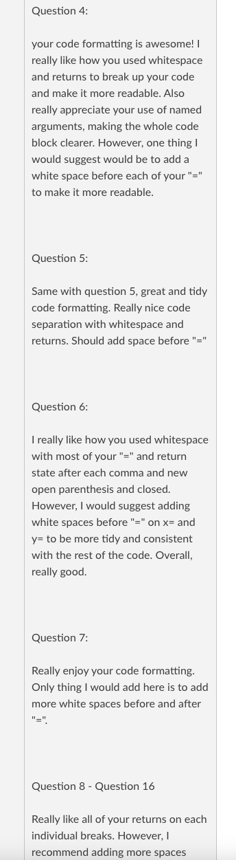
The following is the feedback that I gave that I’m most proud of in one of my peer review. I included an in-depth review of my peer’s general code formatting. I also gave some suggestions on how to write more tidy codes like adding more spaces between "=" and adding more return statements after "," .

Before my discussion with Dr. Theobold, I didn’t fully understand the Developer/Coder protocol established for our team. My collaboration with my partner was largely one-sided—I often took the lead, typing out solutions and implementing my ideas without much input from them. This approach limited my partner’s opportunities to engage and grow as a developer. After our conversation, I made a conscious effort to alternate roles more consistently, ensuring we both contributed by actively listening, discussing, and sharing our ideas as Developers and Coders. This shift allowed for a more balanced and productive collaboration.