Coding a One-way ANOVA – Final Project Work Day

Upcoming Deadlines

• Lab 7 revisions are due by this Friday (by midnight)
• Lab 8 revisions are due next Friday
• Statistical Critique 2 revisions are due next Friday

One Round of Revisions

There is only time for one round of revisions for Lab 8 and Stat Critique #2, so please make sure you feel confident in your revisions! Feel free to stop by my office or schedule a time to chat about your revisions!

Also, please don’t forget reflections!

Additional Revision

If you missed the deadline for the revisions on any assignment, I’m reopening the revisions.

You are permitted to submit one additional assignment for revisions, if you missed the original deadline for the revisions.

Coding a One-way ANOVA

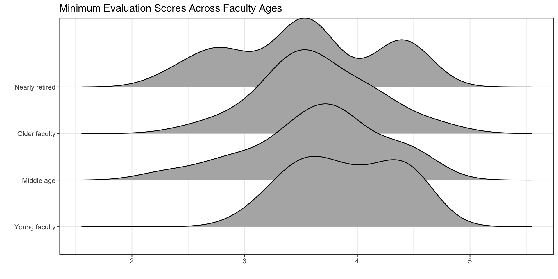
Visualizations – Density Ridges

ggplot(data = <NAME OF DATASET>, 
       mapping = aes(x = <NAME OF NUMERICAL VARIABLE>, 
                     y = <NAME OF CATEGORICAL VARIABLE>)
       ) + 
  geom_density_ridges()+
  labs(x = "<TITLE FOR THE X-AXIS>", 
       y = "<TITLE FOR THE Y-AXIS>")

Revisit the code you wrote for Question 8 of Lab 3

Choosing a Statistical Model

Everyone will fit two one-way ANOVA models — one model for each explanatory variable!

• You will need to choose whether to use a theory-based method or a simulation-based method.
• Your choice is based on the normality condition.

Theory-based Method

To fit a theory-based ANOVA, you use the following code:

my_model <- lm(<NAME OF RESPONSE VARIABLE> ~ <NAME OF EXPLANATORY VARIABLE>, 
                data = <NAME OF DATASET>)

anova(my_model) %>%
  tidy()

Only use if normality is not violated!

If you look at your density ridge plots and you believe the normality condition is violated, you should not use a theory-based method!

Simulation-based Method

To fit a simulation-based ANOVA, you need to carry out the following steps:

1. find the observed statistic
2. simulate statistics that could have happened if the null was true
3. visualize the distribution of simulated statistics (your permutation distribution)
4. calculate the p-value for your observed statistic

2 levels versus 3 levels

If you categorical variable has two levels, you need to use a "diff in means" statistic, not an F-statistic!

Discussion – A New Component

Are your p-values trustworthy?

Inspect the conditions of your model!

Independence of Observations

Consider how the data were collected!

Normality of Residuals (Responses)

Use the density ridge plots!

Equal Variances of Each Group

Use the density ridge plots!

Study Limitations

Same questions as last project!

Extra Features

Do you want to know the sample size in each group?

evals_small %>%
  count(age_cat) 

# A tibble: 4 × 2
  age_cat            n
  <fct>          <int>
1 Young faculty     18
2 Middle age        22
3 Older faculty     40
4 Nearly retired    14

Constant Variance

The constant variance condition is really important when the sample sizes of each group are quite different.

Do you want to change the grey background of your plots?

ggplot(data = evals_small, 
       mapping = aes(y = age_cat, x = min_eval)) + 
  geom_density_ridges() + 
  labs(title = "Minimum Evaluation Scores Across Faculty Ages", 
       y = "",
       x = "") +
  theme_bw()

Do you want to change the grey background of your plots?

Do you want to know the variances for each group?

evals_small %>% 
  group_by(age_cat) %>% 
  summarize(
    var = var(min_eval, na.rm = TRUE)
            ) 

age_cat	var
Young faculty	0.2111438
Middle age	0.3425974
Older faculty	0.2461282
Nearly retired	0.4610989

Constant Variance

A rule that is sometimes used is if the largest variance (0.461) divided by the smallest variance (0.211) is more than 3, then there is evidence of non-equal variance.