Confidence Intervals – Real Life Sampling Distributions
Course Updates
- Lab 4 revisions are due on Friday (May 16)
- Lab 3 second revisions are due on Friday (May 16)
- Midterm Projects will be graded by Sunday (May 18)
Don’t forget reflections!
If your reflections are not present by the deadline for revisions, your revisions are not eligible to be regraded. Please don’t forget your reflections!
What if I only have one sample?
Approximate the variability you’d expect to see in other samples!
Bootstrapping!
A Bootstrap Resample
- Assumes the original sample is “representative” of observations in the population.
- Uses the original sample to generate new samples that might have occurred with additional sampling.
We can use the statistics from these bootstrap resamples to approximate the true sampling distribution!
Why do we want a sampling distribution?
Estimating a population parameter
- We are interested in knowing how a statistic varies from sample to sample.
- Knowing a statistic’s behavior helps us make better / more informed decisions!
- This helps us estimate what values are more or less likely for the population parameter to have.
Confidence Intervals
Capture a range of plausible values for the population parameter.
Are more likely to capture the population parameter than a point estimate.
How do I get this plausible range of values?
Bootstrapping!
- From your original sample, resample with replacement the same number of times as your original sample.
This is your bootstrap resample.
- Repeat this process many, many times.
- Calculate a numerical summary (e.g., mean, median) for each bootstrap resample.
These are your bootstrap statistics
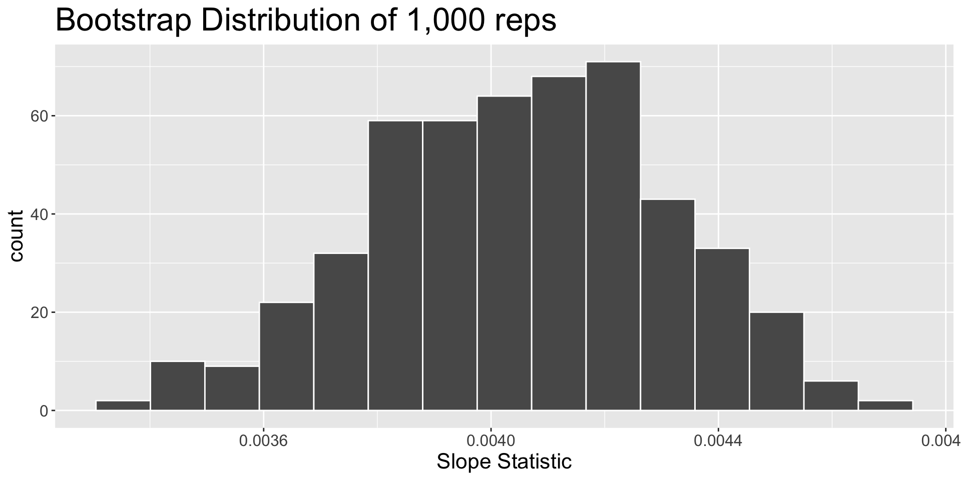
Bootstrap Distribution
a distribution of the bootstrap statistics from every bootstrap resample
Displays the variability in the statistic that could have happened with repeated sampling.
Approximates the true sampling distribution!
Penguins!
Statistic: \(\beta_1\)
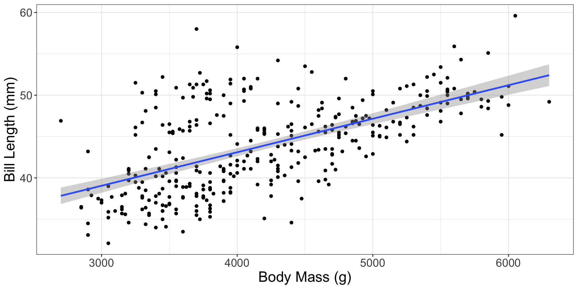
The relationship between penguin’s bill length and body mass for all penguins in the Palmer Archipelago
In this sample of 344 penguins…
\[\widehat{\text{bill length}} = 26.899 + 0.004 \times \text{body mass}\]
What slope could have happened in a different sample of penguins?
Generating bootstrap resamples and calculating bootstrap statistics
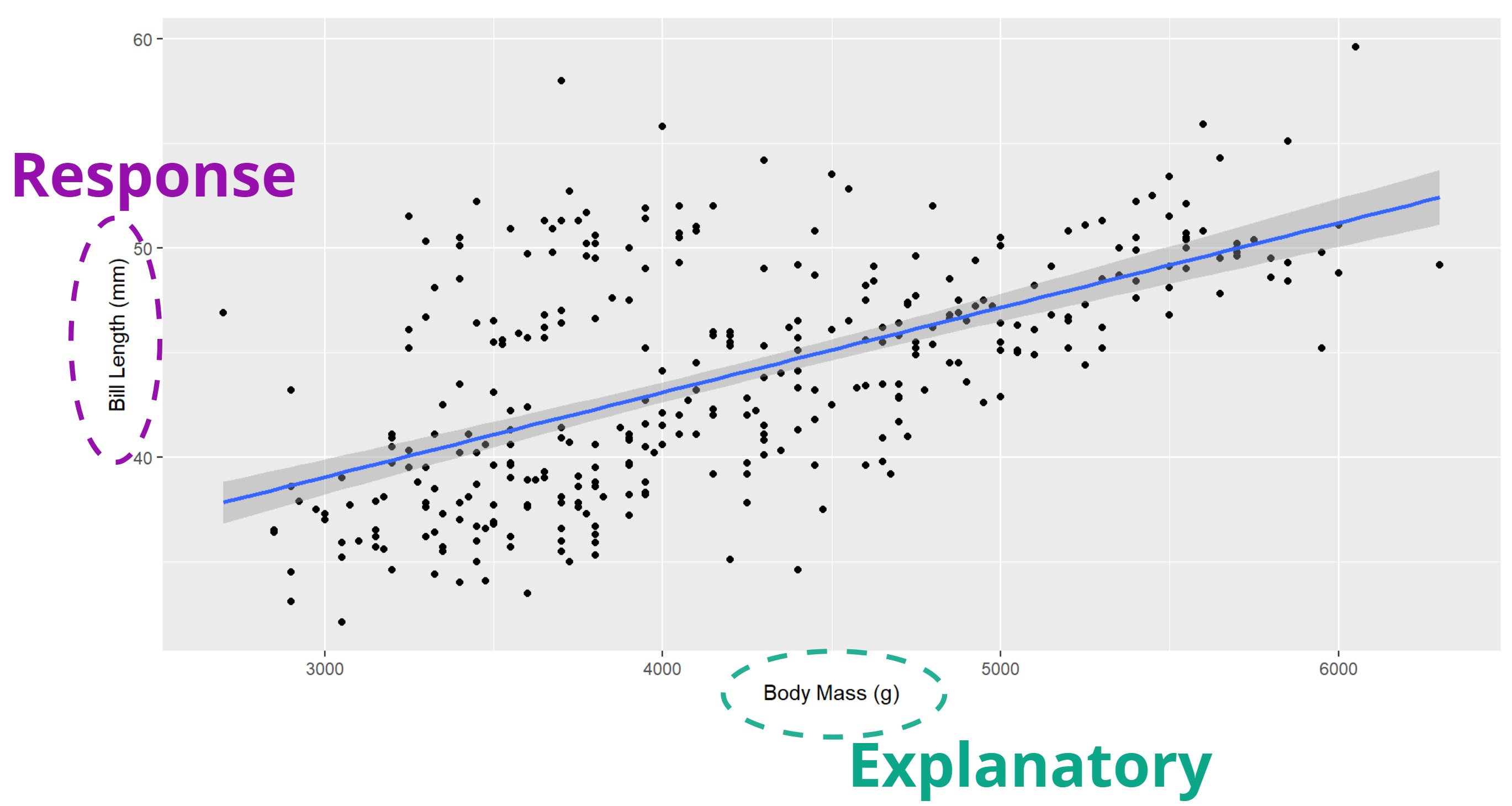
Step 1: specify() your response and explanatory variables
Step 2: generate() bootstrap resamples
Step 3: calculate() the statistic of interest
Step 1: Specify your variables!
Step 2: Generate your resamples!
reps – the number of resamples you want to generate
"bootstrap" – the method that should be used to generate the new samples
Your turn!
Why do we resample with replacement when creating a bootstrap distribution?
When we resample with replacement from our original sample what are we assuming about the original sample?
Step 3: Calculate your statistics!
"slope" – the statistic of interest
The final product
A plausible range of values for \(\beta_1\)
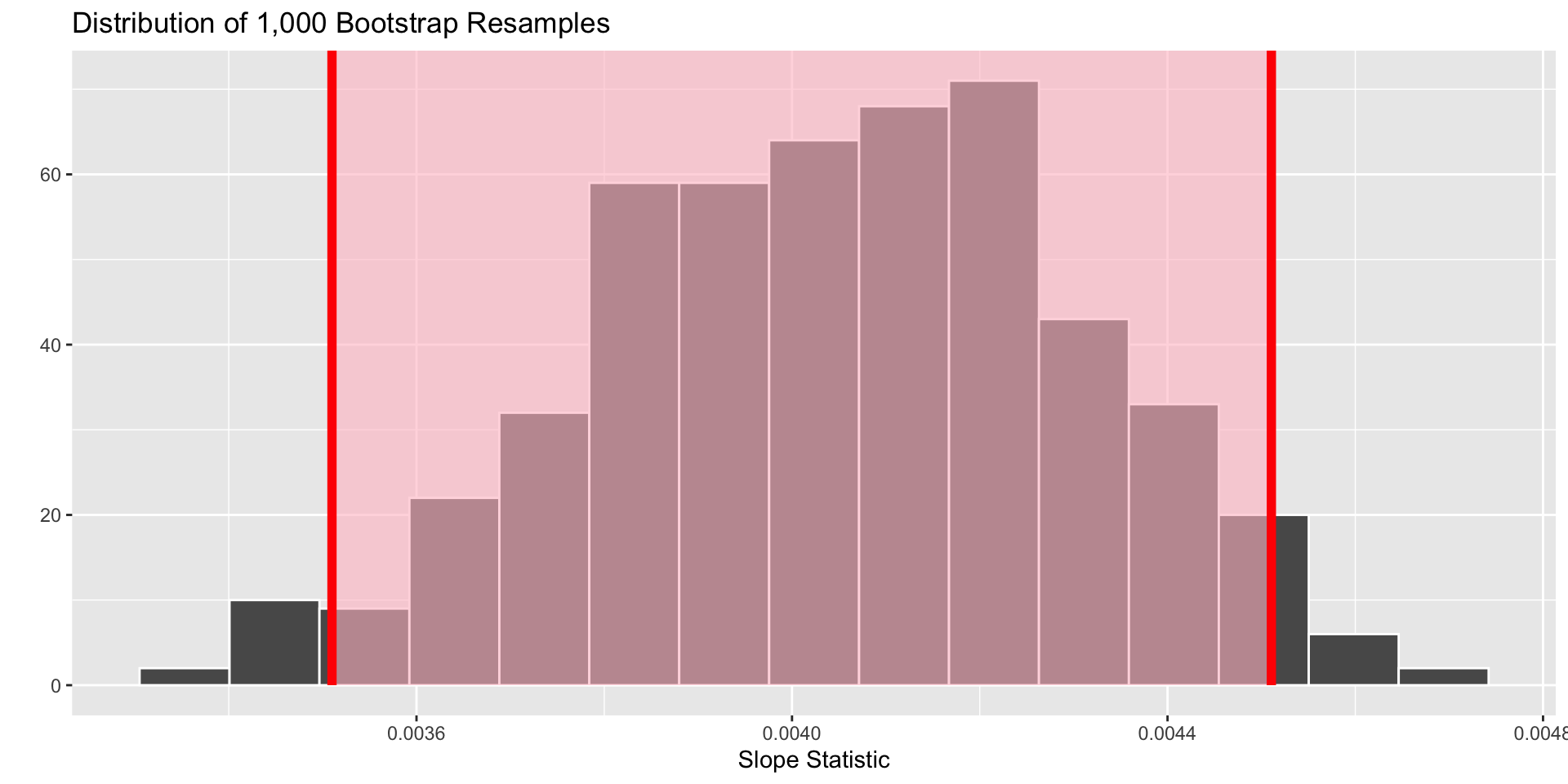
The 95% confidence interval is…
| Lower Bound | Upper Bound |
|---|---|
| 0.00351 | 0.00451 |
What do we hope is captured by this interval?
How do we interpret this interval?
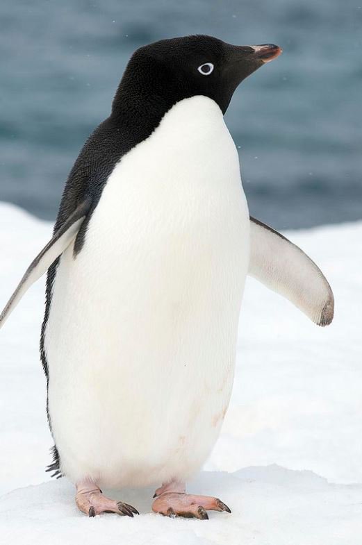
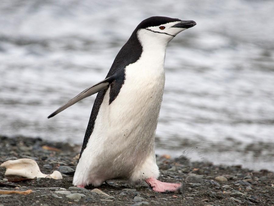
“We are 95% confident the slope of the relationship between bill length and body mass for all Adelie, Chinstrap, and Gentoo penguins in the Palmer Archipelago is between 0.00355 and 0.00453.
“For every 1000 gram (~2.2lbs) increase in a penguin’s body mass, we are 95% confident the length of an Adelie, Chinstrap, or Gentoo penguins’s bill will increase between 3.55 and 4.53mm.
Classic interpretation mistakes
“There is a 95% probability that \(\beta_1\) is between 0.00355 and 0.00453.”
“We are 95% confident the sample statistic is in our interval.”
Scaling to Multiple Linear Regression
How does the relationship between bill length and body mass change based on a penguin’s sex?
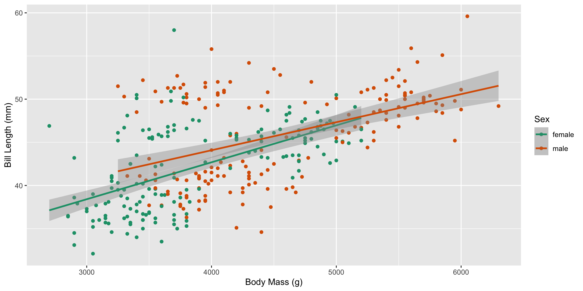
What changes?
The original sample of 344 penguins were broken down into the following groups (plus 11 NA values):
| Sex | Sample Size |
|---|---|
| female | 165 |
| male | 168 |
Before we resampled with replacement 344 times.
If we resample with replacement 333 times, are we guaranteed to get 165 female penguins and 168 male penguins in each sample?
Getting our Observed Statistic
Step 1: Fitting our Model
Syntax changes
When we have multiple explanatory variables, we need to use the “tilde” (~) syntax to specify our model. We also use the fit() function instead of the calculate() function.
Getting our Observed Statistic
Step 2: Finding our Statistic
| term | estimate |
|---|---|
| intercept | 25.5713814 |
| body_mass_g | 0.0042787 |
| sexmale | 5.5160611 |
| body_mass_g:sexmale | -0.0010301 |
Which statistic measures how different the slopes are between male and female penguins?
Generating Bootstrap Fits
Obtaining a Bootstrap Confidence Interval
How do we interpret this interval?
| Lower Bound | Upper Bound |
|---|---|
| -0.0019812 | -0.0001181 |
We are 90% confident that the for every 1,000 gram increase in a penguin’s body mass (~2.2lbs), the length of a male penguin’s bill is between 0.118 and 1.98mm shorter than a female penguin’s bill.
To Do List by Wednesday
- Hypothesis test reading guide
- Hypothesis test concept quiz
- Confidence interval R tutorial
- Hypothesis test R tutorial