Week 3 Day 2

STAT 313

Lab 1 Revisions Due Friday

Ethical Considerations with Categorical Variables

Choosing What to Measure - Gender

Keller et al. (2017) designed a study to examine whether a community-based suicide prevention project could increase willingness to seek professional help for suicidal ideation among eastern Montana youth.

Students attending the Let’s Talk theater workshop, were asked to report their gender, race, and age.

Choosing What to Measure - Gender

Researchers provided students with the following question:

What is your gender?

Male, Female, Other

What information are the researchers missing?

Why is that information important?

Choosing What to Measure - Sex

\(\beta\) blockers have been shown to improve survival in patients with congestive heart failure. These medicines block the effects of the hormone epinephrine (adrenaline). Research suggests that beta blockers have a differing effect for individuals with high levels of estrogen (Khan and Movahed 2000).

Choosing What to Measure - Sex

The intake form for a local heart clinic asks the following question:

What is sex were you assigned at birth?

Male, Female, Other

What information are the doctors missing?

Why is that information important?

Choosing What to Measure - Race

Every year, the US publishes a large dataset on the public birth records for babies born that year. These data contain information about the baby, the pregnancy, and the birth parent(s).

Choosing What to Measure - Race

Looking at the births14 dataset, the race of the mother was classified as:

• white
• nonwhite

What information is missing?

Why is that information important?

Lab 3

Today’s Data

The and_vertebrates dataset contains length and weight observations for Coastal Cutthroat Trout and two salamander species (Coastal Giant Salamander, and Cascade Torrent Salamander) in previously clear cut (c. 1963) and old growth coniferous forest sections of Mack Creek in HJ Andrews Experimental Forest, Willamette National Forest, Oregon.

Research Question

Are there differences in fish biomass between clear cut and old growth sections of the HJ Andrews Forest?

Clear Cutting

In the 1950s and 60s researchers clear cut sections of the HJ Andrews forest to research the efficiency of forest operations, including logging, road building, and forest regeneration.

Data Layout

year	sitecode	section	reach	pass	unitnum	unittype	vert_index	pitnumber	species	length_1_mm	length_2_mm	weight_g	clip	sampledate	notes
2013	MACKOG-U	OG	U	1	14	P	1	NA	Cascade torrent salamander	41	71	NA	NONE	2013-09-06	NA
2017	MACKCC-L	CC	L	1	2	SC	29	NA	Cascade torrent salamander	39	67	1.3	NONE	2017-09-05	NA
1995	MACKCC-L	CC	L	1	1	P	12	NA	Coastal giant salamander	67	114	11.1	NONE	1995-08-30	NA
2003	MACKCC-U	CC	U	1	9	C	63	NA	Coastal giant salamander	85	151	NA	NONE	2003-09-02	ADULT
1998	MACKOG-M	OG	M	1	5	C	2	NA	Cutthroat trout	121	NA	NA	LV	1998-09-02	NA
2007	MACKOG-U	OG	U	1	13	C	74	NA	Cutthroat trout	45	NA	NA	NONE	2007-09-13	NA
1990	MACKCC-L	CC	L	1	3	SC	1	NA	NA	NA	NA	NA	NONE	1990-08-15	not sampled
1995	MACKOG-M	OG	M	1	10	S	1	NA	NA	NA	NA	NA	NONE	1995-08-29	JAM

What are the observations / rows in this dataset?

If you wanted to find the mean mass for Cutthroat trout in each section, what would you do?

Step 1: Remove Salamanders

trout <- filter(and_vertebrates, 
                species == "Cutthroat trout") 

Step 2: group_by() + summarize()

trout %>% 
  group_by(section) %>% 
  summarize(
    mean_mass = mean(weight_g,
                     na.rm = TRUE)
            )

# A tibble: 2 × 2
  section    mean_mass
  <chr>          <dbl>
1 Clear cut       9.38
2 Old growth      8.21

Remember na.rm = TRUE is important if there are missing values!

Are they different?

Forest Section	Mean Biomass
Clear cut	9.380571
Old growth	8.213796

Would you conclude there is a difference in fish biomass between clear cut and old growth sections of the HJ Andrews Forest?

Let’s Make a Visualization!

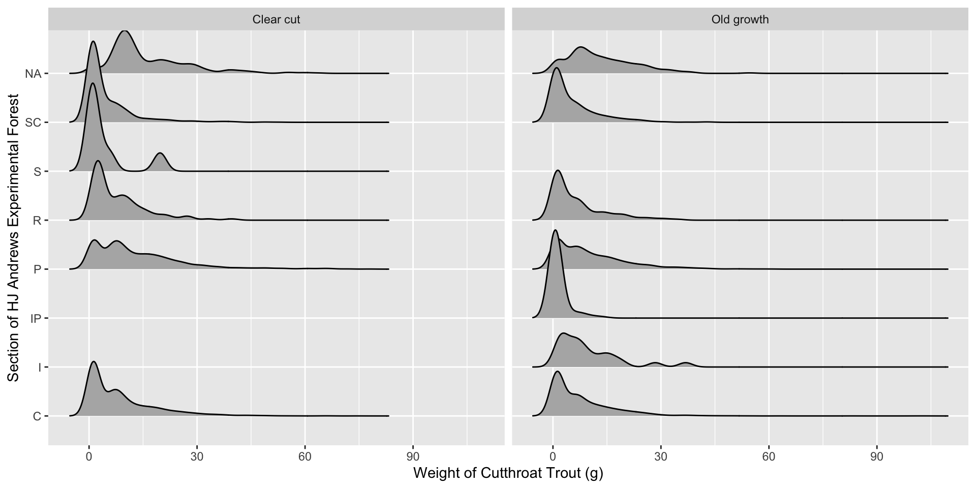
ggplot(data = trout, 
       mapping = aes(x = weight_g, 
                     y = section)
       ) +
  geom_density_ridges() +
  labs(x = "Weight of Cutthroat Trout (g)",
       y = "",
       title = "Length of Salamanders for Different Sections of HJ Andrews Experimental Forest")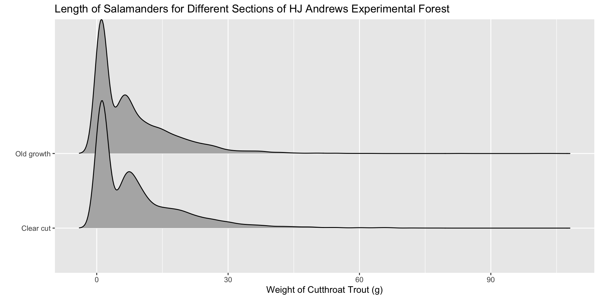 

Are they different?

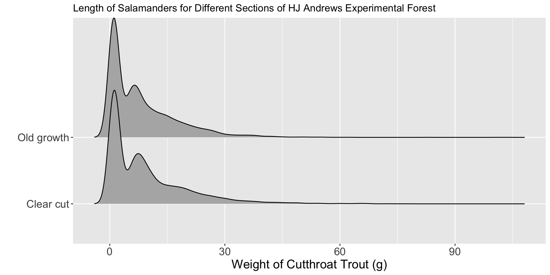
Would you conclude there is a difference in fish biomass between clear cut and old growth sections of the HJ Andrews Forest?

Let’s Add in the Type of Channel

The channels (unittype) of the Mack Creek which were sampled were classified into the following groups:

"C"

"I"

"IP"

"P"

"R"

"S"

"SC"

NA

cascade

riffle

isolated pool

pool

rapid

step (small falls)

side channel

not sampled by unit

If you wanted to find the mean mass for Cutthroat trout for each type of channel in each section, what would you do?

group_by() Multiple Variables

trout %>% 
  group_by(section, unittype) %>% 
  summarize(
    mean_mass = mean(weight_g, 
                     na.rm = TRUE)
            )

# A tibble: 13 × 3
# Groups:   section [2]
   section    unittype mean_mass
   <chr>      <chr>        <dbl>
 1 Clear cut  C             8.47
 2 Clear cut  P            13.4 
 3 Clear cut  R             8.06
 4 Clear cut  S             4.34
 5 Clear cut  SC            4.80
 6 Clear cut  <NA>         16.3 
 7 Old growth C             7.58
 8 Old growth I             9.81
 9 Old growth IP            1.39
10 Old growth P            10.4 
11 Old growth R             6.66
12 Old growth SC            5.38
13 Old growth <NA>         13.4 

Visualization 2.0 – Incorporating Color

ggplot(data = trout, 
       mapping = aes(x = weight_g, 
                     fill = section, 
                     y = unittype)
       ) +
  geom_density_ridges(alpha = 0.5) +
  labs(x = "Weight of Cutthroat Trout (g)", 
       fill = "Section of HJ Andrews \nExperimental Forest", 
       y = "Type of Channel")

Visualization 2.0 – Incorporating Color

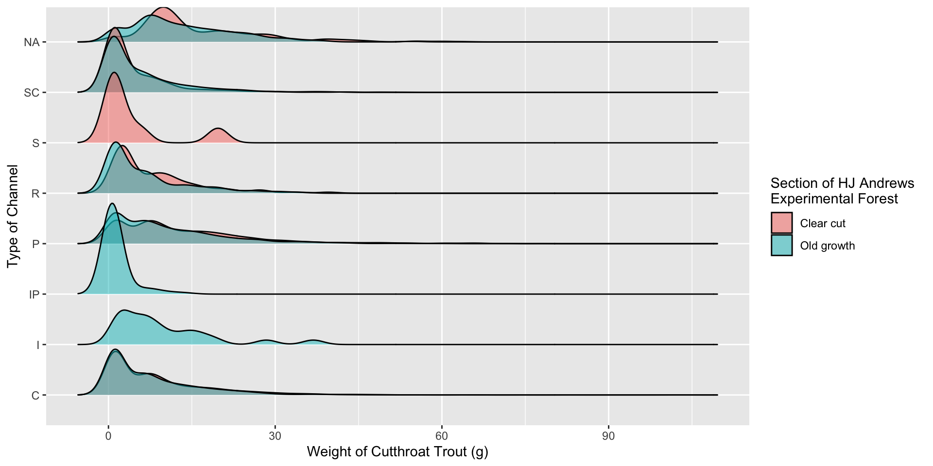
Visualization 2.0 – Incorporating Color

Why put unittype on the y-axis instead of section???

Visualization 2.0 – Incorporating Facets

ggplot(data = trout, 
       mapping = aes(x = weight_g, 
                     y = unittype)) +
  geom_density_ridges() +
  labs(x = "Weight of Cutthroat Trout (g)", 
       y = "Section of HJ Andrews Experimental Forest") +
  facet_wrap(~section)

Visualization 2.0 – Incorporating Facets

Lab 3

Accessing Lab 3

Roles

The person who was not the Recorder last week acts as the Recorder this week (change roles!).

Step 2: The Recorder follows these instructions to copy the Lab 2 project into your group’s workspace

Step 3: Both members open the Lab 3 assignment in your group workspace!

Step 4: Follow the final instructions to activate collaborative editing in the document.

References

Keller, Sarah N., and Timothy Wilkinson. 2017. “Preventing Suicide in Montana: A Community-Based Theatre Intervention.” Journal of Social Marketing 7 (4): 423–40. https://doi.org/10.1108/jsocm-12-2016-0086.

Khan, Nazim Uddin Azam, and Assad Movahed. 2000. “Role of ß Blockers in Congestive Heart Failure.” Congestive Heart Failure 6 (6): 299–312. https://doi.org/10.1111/j.1527-5299.2000.80176.x.