Writing Vector Functions

Thursday, October 30

Today we will…

• Review function basics
• Practice writing functions!
  • [] refresher
  • seq_along()
  • if() and else if() refresher
• PA 7: Writing Functions
• Extra Slides for Lab 7
  • Variable Scope + Environment

Functions

Why write functions?

Functions allow you to automate common tasks!

Writing functions has three big advantages over copy-paste:

1. Your code is easier to read.
2. To change your analysis, simply change one function.
3. You avoid mistakes.

Function Basics

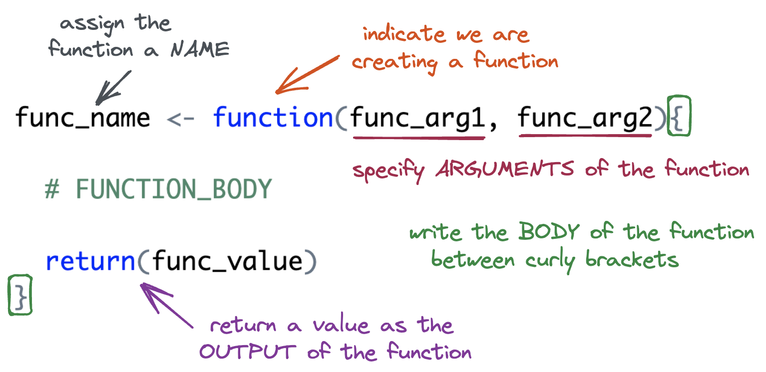
Function Syntax

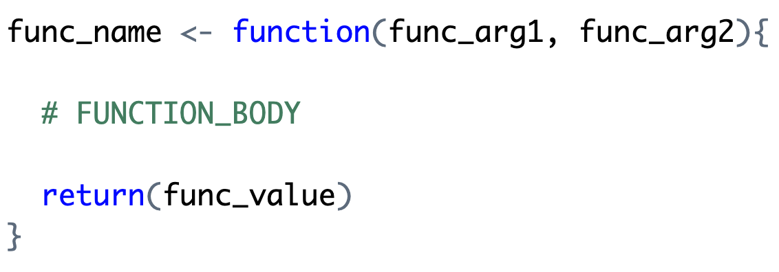
Function Syntax

A (Very) Simple Function

Write a function named add_two() that will add 2 to whatever number is input.

03:00

Compare Your Function with Your Neighbor

In what ways are your functions the same? In what ways do they differ?

Function Names

The name of the function is chosen by the author.

add_two <- function(x){
  
  return(x + 2)

}

Function names have no inherent meaning.

The name you give to a function does not affect what the function does.

add_three <- function(x){
  return(x + 7)
}

add_three(5)

[1] 12

Function Arguments

The argument(s) of the function are chosen by the author.

• Arguments are how we pass external values into the function.
• They are temporary variables that only exist inside the function body.

• We give them general names:
  • x, y, z – vectors
  • df – data frame
  • i, j – indices

add_two <- function(x){
  return(x + 2)
}

Function Arguments

What if we wanted to write a more general function, named add_something(). The function would take two inputs:

1. x the vector to add to
2. something the value to add to x

How would your function change?

02:00

Function Arguments

• Required Arguments
• Optional Arguments

If we do not supply a default value when defining the function, the argument is required when calling the function.

add_something <- function(x, something){
  x + something
}

add_something(x = 2, 
              something = 3)

[1] 5

add_something(x = 2)

Error in add_something(x = 2): argument "something" is missing, with no default

If we supply a default value when defining the function, the argument is optional when calling the function.

add_something <- function(x, something = 2){
  return(x + something)
}

add_something(x = 5, 
              something = 6)

[1] 11

If a value is not supplied, something defaults to 2.

add_something(x = 5)

[1] 7

Optional Arguments

A lot of the functions we’ve been working with so far actually have a lot of optional arguments:

mean(x, 
     trim = 0, 
     na.rm = FALSE, ...)

max(..., na.rm = FALSE)
min(..., na.rm = FALSE)

geom_point(
  mapping = NULL,
  data = NULL,
  stat = "identity",
  position = "identity",
  ...,
  na.rm = FALSE,
  show.legend = NA,
  inherit.aes = TRUE
)

Body: { }

The body of the function is where the action happens.

• The body must be specified within a set of curly brackets.
• The code in the body will be executed (in order) whenever the function is called.

add_something <- function(x, something = 2){
  x + something
}

Output: Last Value

Your function will give back what would normally print out…

add_something <- function(x, something = 2){
  x + something
}

7 + 2

[1] 9

add_something(7)

[1] 9

…but some of us might prefer an explicit return().

Output: return()

If you are coming to R from a background in Python, C, or Java then an explicit return may feel more natural to you.

add_something <- function(x, something = 2){
  return(x + something)
}

Function Style – Using return()s

“Only use return() for early returns. Otherwise, rely on R to return the result of the last evaluated expression.”

safe_square <- function(x) {
  if (!is.numeric(x)) return(NA)
  x^2
}

Explicit Returns vs. Implicit Returns

✅ Pros of Using return()

• Clarity and explicit intent
• Early returns / branching logic
• Consistency with other languages

⚠️ Cons of Using return()

• More typing / slightly less idiomatic use of R
• Can be overused in simple functions
• Can complicate control flow unnecessarily

✅ Pros of Implicit Return (no return())

• Concise and idiomatic
• Encourages “last expression” thinking

⚠️ Cons of Implicit Return

• Less obvious for beginners
• Harder to do early exits

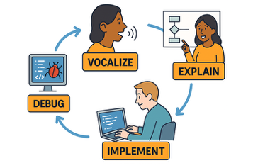
General Function Writing Advice

When you have a concept that you want to turn into a function…

1. Write a simple example of the code without the function framework.

2. Generalize the example by assigning variables.

3. Write the code into a function.

4. Call the function on the desired arguments

This structure allows you to address issues as you go.

Let’s Practice

Base R Refresher

• We can extract components of a vector using [ ]
  • The inputs can be:
    • logical values (TRUE, FALSE)
    • indices (e.g., 1, 2, 3)

• We can grab the indices of a vector using the seq_along() function

x <- 15:25
x

 [1] 15 16 17 18 19 20 21 22 23 24 25

seq_along(x)

 [1]  1  2  3  4  5  6  7  8  9 10 11

above_average()

Goal: Keep only the elements of x greater than the mean.

Fill in the code to create a function named above_average(). The function should keep only the elements of x greater than the mean.

above_average <- function(x) {
  # Step 1: Compute mean of x
  
  
  # Step 2: Subset x to keep only values > mean
  
  
  # Step 3: Return the result
  
}

05:00

Option 1: Using Logical Values

Step 1: Find locations where values of x are larger than the mean

x > mean(x)

 [1] FALSE FALSE FALSE FALSE FALSE FALSE  TRUE  TRUE  TRUE  TRUE  TRUE

Step 2: Use this output to extract the desired values from x

x[x > mean(x)]

[1] 21 22 23 24 25

Step 3: Make a function

above_average <- function(x) {
  x[x > mean(x)]
}

Option 2: Using Indices

Step 1: Find indices where values of x are larger than the mean

which(x > mean(x))

[1]  7  8  9 10 11

Step 2: Use this output to extract the desired values from x

x[which(x > mean(x))]

[1] 21 22 23 24 25

Step 3: Make a function

above_average <- function(x) {
  x[which(x > mean(x))]
}

every_third()

Goal: Return every third element from a vector.

Write down the steps you would need to create a function named every_third() that takes in a vector and returns every third element from that vector (i.e., indices 1, 4, 7, 10, etc.).

Think about:

• What inputs the function should take.
• How to identify which positions in the vector are “every third.”
• How to select those elements from the vector.

03:00

Generate Indices

Represent the indices (positions) of each element of x.

x

 [1] 15 16 17 18 19 20 21 22 23 24 25

seq_along(x)

 [1]  1  2  3  4  5  6  7  8  9 10 11

Identify Every Third Position

Identify which positions are “every third.”

index	Remainder (index %% 3)	Keep?
1	1	✅
2	2	❌
3	0	❌
4	1	✅
5	2	❌
6	0	❌
7	1	✅

Identify Every Third Position

Identify which positions are “every third.”

seq_along(x) %% 3 == 1

 [1]  TRUE FALSE FALSE  TRUE FALSE FALSE  TRUE FALSE FALSE  TRUE FALSE

Subset x

Grab the elements of x we want to keep.

x

 [1] 15 16 17 18 19 20 21 22 23 24 25

x[ 
  seq_along(x) %% 3 == 1
]

[1] 15 18 21 24

Make it into a function!

every_third <- function(x) {
  
  x[ 
  seq_along(x) %% 3 == 1
  ]

  }

PA 7: Writing Functions

PA 7

You will write several small functions, then use them to unscramble a message. Many of the functions have been started for you, but none of them are complete as is.

This activity will require knowledge of:

• Function syntax
• Optional and required arguments
• Modulus division (and remainders)
• Using [] and logical values to extract elements of a vector
• Negating logical statements
• if () & else if() statements

None of us have all these abilities. Each of us has some of these abilities.

Pair Programming Expectations

External Resources

During the Practice Activity, you are not permitted to use Google or ChatGPT for help.

You are permitted to use:

• today’s handout,
• the course slides,
• the base R cheatsheet, and
• the course textbook

Submission

Submit the name of the television show the six numbers are asssociated with.

• Each person will input the full name of the TV show into the PA 7 quiz.
• The person who last occupied the role of Typer will submit the link to your group’s Colab notebook.
  • Please don’t forget to put your names at the top!

5-minute break

Team Assignments - 9am

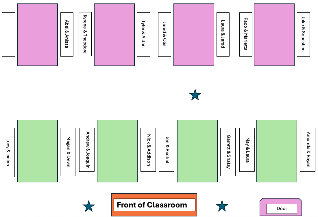
The partner who has the most siblings starts as the Talker!

Team Assignments - 12pm

The partner who has the most siblings starts as the Talker!

Lab 7 Bonus Slides

Lab 7 & Challenge 7: Functions + Fish

Input Validation

When a function requires an input of a specific data type, check that the supplied argument is valid.

• stopifnot()
• if() + stop()
• Multiple validations

add_something <- function(x, something){
  stopifnot(is.numeric(x))
  return(x + something)
}

add_something(x = "statistics", something = 5)

Error in add_something(x = "statistics", something = 5): is.numeric(x) is not TRUE

add_something <- function(x, something){
  if(!is.numeric(x)){
    stop("Please provide a numeric input for the x argument.")
  }
  return(x + something)
}

add_something(x = "statistics", something = 5)

Error in add_something(x = "statistics", something = 5): Please provide a numeric input for the x argument.

How would you modify the previous code to validate both x and something?

Meaning, the function should check if both x and something are numeric.

Multiple Validations

• Option 1: if() + stop()
• Option 2: stopifnot()

add_something <- function(x, something){
  if(!is.numeric(x) | !is.numeric(something)){
    stop("Please provide numeric inputs for both arguments.")
  }
  return(x + something)
}

add_something(x = 2, something = "R")

Error in add_something(x = 2, something = "R"): Please provide numeric inputs for both arguments.

add_something <- function(x, something){
  stopifnot(is.numeric(x), is.numeric(something))
  return(x + something)
}

add_something(x = 2, something = "R")

Error in add_something(x = 2, something = "R"): is.numeric(something) is not TRUE

Variable Scope + Environment

Variable Scope

The location (environment) in which we can find and access a variable is called its scope.

• We need to think about the scope of variables when we write functions.
• What variables can we access inside a function?
• What variables can we access outside a function?

Global Environment

• The top right pane of Rstudio shows you the global environment.
  • This is the current state of all objects you have created.
  • These objects can be accessed anywhere.

Function Environment

• The code inside a function executes in the function environment.
  • Function arguments and any variables created inside the function only exist inside the function.
    • They disappear when the function code is complete.
• What happens in the function environment does not affect things in the global environment.

Function Environment

We cannot access variables created inside a function outside of the function.

add_two <- function(x) {
  my_result <- x + 2
  return(my_result)
}

add_two(9)

[1] 11

my_result

Error in eval(expr, envir, enclos): object 'my_result' not found

Name Masking

Name masking occurs when an object in the function environment has the same name as an object in the global environment.

add_two <- function(x) {
  my_result <- x + 2
  return(my_result)
}

my_result <- 2000

The my_result created inside the function is different from the my_result created outside.

add_two(5)

[1] 7

my_result

[1] 2000

Dynamic Lookup

Functions look for objects FIRST in the function environment and SECOND in the global environment.

• If the object doesn’t exist in either, the code will give an error.

add_two <- function() {
  return(x + 2)
}

add_two()

 [1] 17 18 19 20 21 22 23 24 25 26 27

• If it doesn’t exist in the function environment, then it will look in the global environment

x <- 10

add_two()

[1] 12

It is not good practice to rely on global environment objects inside a function!