get_shared_birthdays <- function(n = 50){

  bday_data <- tibble(person = 1:n,
                      bday   = sample(1:365,
                                      size = n,
                                      replace = TRUE)
                      )
}Simulating Probabilities & Datasets
Today we will…
- Reminder about Lab 8 (and 9 and 10) Code Review
- Thinking through a probability simulation task
- Introduce Lab 9
- Refresher on linear regression
- Tools for extracting elements from a regression
- Survey on Experiences in STAT 331 / 531
- Work time!
Don’t forget to complete your Lab 8 code review!
Don’t forget to complete your Lab 8 code review!
Make sure your feedback follows the code review guidelines.
Insert your review into the comment box!
Lab 9: Simulating Probabilities
The Birthday Problem
Simulate the approximate probability that at least two people have the same birthday (same day of the year, not considering year of birth or leap years).
Writing a function to…
- simulate the birthdays of 50 people.
- count how many birthdays are shared.
- return whether or not a shared birthday exists.
Step 1 – simulate the birthdays of 50 people
Why did I set replace = TRUE for the sample() function?
Step 2 – count how many birthdays are shared
Step 3 – return whether or not a shared birthday exists
What type of output is this function returning?
Using Function to Simulate Many Probabilities
Use a map() function to simulate 1000 datasets.
Lab 9: Simulating Confidence Interval Coverage Rates
Simple Linear Regression (SLR)
If we assume the relationship between \(x\) and \(y\) takes the form of a linear function…
\[ response = intercept + slope \times explanatory + noise \]
SLR Model Notation
In Statistics, there are two types of models—the population model and the fitted (sample) model.
Population Regression Model
\(y_i = \beta_0 + \beta_1 x_i + \epsilon_i\)
where \(\epsilon_i \sim N(0, \sigma)\) is the random noise.
Fitted Regression Model
\(\widehat{y}_i = \widehat{\beta}_0 + \widehat{\beta}_1 x_i\)
where \(\widehat{}\) indicates the value was estimated.
Fitting an SLR Model
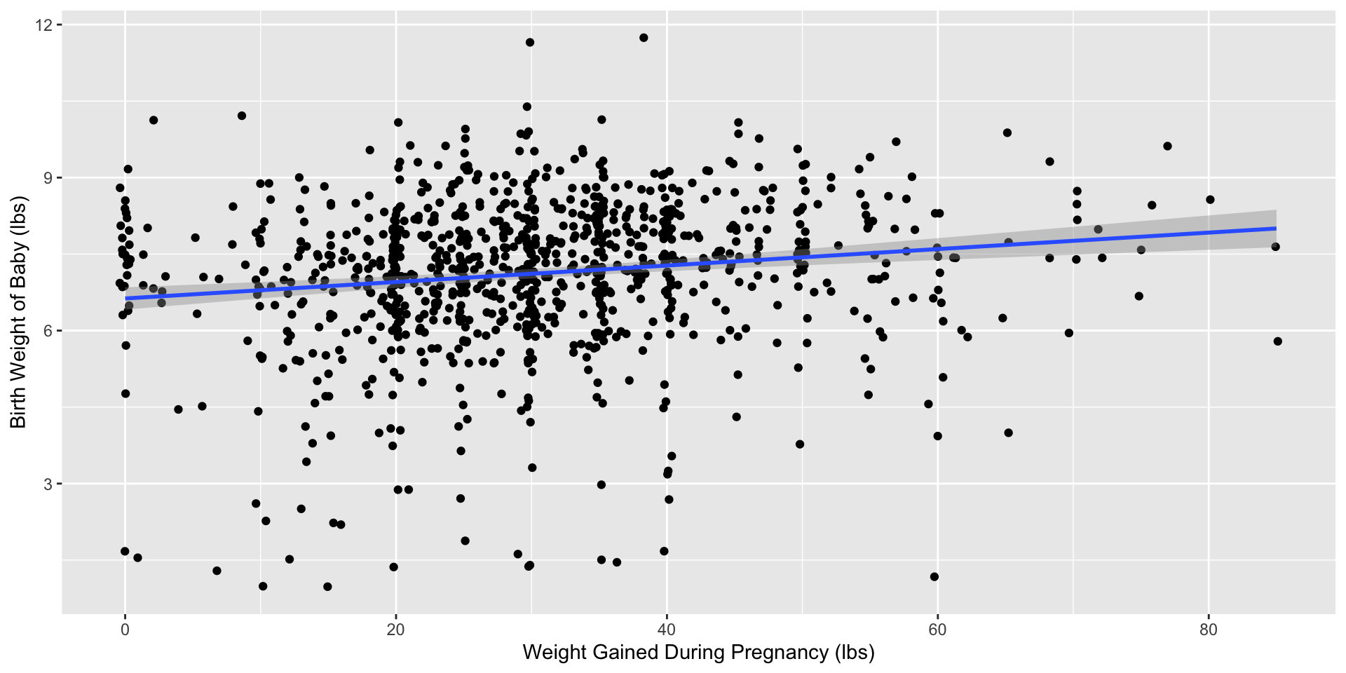
Regress baby birthweight (response variable) on the pregnant parent’s weight gain (explanatory variable).
- We are assuming there is a linear relationship between how much weight the parent gains and how much the baby weighs at birth.
Model Outputs
Call:
lm(formula = weight ~ gained, data = ncbirths)

Residuals:
    Min      1Q  Median      3Q     Max
-6.4085 -0.6950  0.1643  0.9222  4.5158

Coefficients:
            Estimate Std. Error t value Pr(>|t|)
(Intercept)  6.63003    0.11120  59.620  < 2e-16 ***
gained       0.01614    0.00332   4.862 1.35e-06 ***
---
Signif. codes:  0 '***' 0.001 '**' 0.01 '*' 0.05 '.' 0.1 ' ' 1

Residual standard error: 1.474 on 971 degrees of freedom
  (27 observations deleted due to missingness)
Multiple R-squared:  0.02377,   Adjusted R-squared:  0.02276
F-statistic: 23.64 on 1 and 971 DF, p-value: 1.353e-06| term | estimate | std.error | statistic | p.value | conf.low | conf.high |
|---|---|---|---|---|---|---|
| (Intercept) | 6.6300336 | 0.1112054 | 59.619718 | 0.0e+00 | 6.4469423 | 6.8131248 |
| gained | 0.0161405 | 0.0033195 | 4.862253 | 1.4e-06 | 0.0106751 | 0.0216059 |
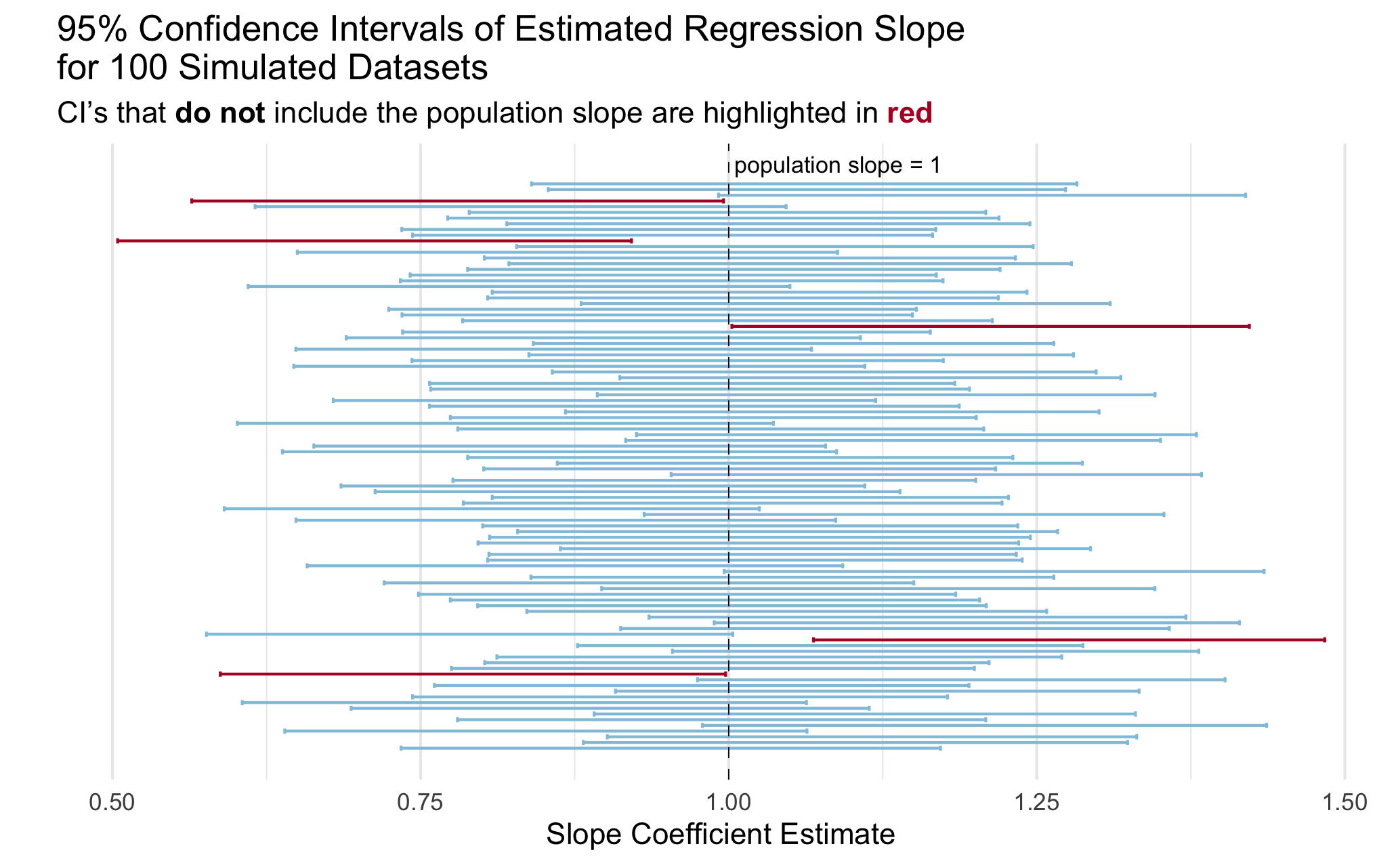
Confidence Level
You can change the confidence level for the confidence interval in the conf.level argument!
Grabbing Model Outputs
Our Goal
Lab 8 Revisions
Lab 8 Revisions
Only problems receiving a growing can be submitted for additional feedback!
I have left many of you comments on changes to make to your code that I trust you can do on your own!
Lab 8 Feedback
Q1: How can you make your code more clear? Argument names?
Q1: How can you make your code more robust? Using ~ to define a function? Using .x to indicate where the input should go?
Q1 & Q3: How can you incorporate input checks into your function? Checking if the input is a data frame? Checking if the variables are the right data type? Checking if the variables are included in the data frame?
Q5: Can you give your function a name that describes what it does? (e.g., make_filled_barplot(), make_colored_scatterplot())
Q5: We haven’t learned paste() or paste0() in this class! What functions have we learned that executed this process?
Survey on Experiences in STAT 331 / 531
Anonymous Google Form: https://forms.gle/YzZWe2oJZ5eWyTbRA
If we get an 85% completion rate I will bring doughnuts to class next Thursday!