df_songs['Mode'] = (
  df_songs['Mode']
  .replace({1: 'Major', 0: 'Minor'})
)Combining Datasets
Plan for Today
What’s ahead with Final Projects
Debrief on Lab 7
- Why clean a variable
- Categorical variables vs. one-hot encoded variables
- Model errors
- Coefficient interpretation
3. Discuss different types of joins
- Keys
- The
merge()function - Joining on multiple keys
- Joining on keys with different names
- Different types of joins
Final Project
Visualizations
Your final poster will contain two (not three, not four) visualizations.
- A visualization which addresses your primary research question.
- A visualization which addresses your secondary research question.
- At least one plot must include 3+ variables.
- Both plots must use non-default colors.
- Both plots should follow the visualization “best practices” outlined in the project resources.
Data Models
Fit a model(s) to the data to address your primary and secondary research questions. You are expected to explicitly state the modeling choices you made and the results of the model(s) you fit.
The following are minimum criteria for the model(s) you fit to your data:
- Include a model covered after the midterm exam (KNN, logistic regression, linear regression, decision tree, k-means).
- Use cross-validation to estimate the testing error of the model.
- Choose a “meaningful” model metric to summarize the fit of a model.
Lab 7 Debrief
Cleaning Variables
What does a Mode of 0 represent?
How did I know that 0 represented a minor key?
The data documentation!
Obtaining Coefficients for Every Variable Level
Even if you converted TimeSignature and Mode into categorical / string variables, you will not get coefficient estimates for every level of these variables.
Q: What do you get?
A: Adjustments for each group relative to the “baseline” group.
Q: What group is the “baseline” group?
A: The group that comes first alphabetically (has the lowest ASCII representation).
Obtaining Coefficients for Every Variable Level
How do you get values for every level of a categorical variable?
Penalized Logistic Regression is the Default!
Model Error versus Testing Error
What is the accuracy of this model?
this model represents the errors of the model that was fit to the training data, where we know the value of the target variable
Cross-validation is not necessary here!
If you were to use this model to predict, what precision would you expect to get?
predicting involves “testing” data, where we don’t know the value of the target variable
Cross-validation is necessary here!
Interpreting Coefficents
Each coefficient is associated with the change in the log-odds of a song containing explicit lyrics.
TimeSignature_1: 1.536751
A 1/4 time signature is associated with an increase of 1.53 in the log-odds of a song containing explicit lyrics.
Speechiness: 0.963213
An increase of speechiness by 1 standard devation above the mean (making the song almost entirely made up of spoken words) is associated with an increase of 0.96 in the log-odds of a song containing explicit lyrics.
Joining Datasets
Example: Planes and Flights
Sometimes, information is spread across multiple data sets.
For example, suppose we want to know which manufacturer’s planes made the most flights in 2013.
Example: Information on Flights
One data set contains information about flights from January to September 2013…
        year  month  day  ...  hour  minute             time_hour
0       2013      1    1  ...     5      15  2013-01-01T10:00:00Z
1       2013      1    1  ...     5      29  2013-01-01T10:00:00Z
2       2013      1    1  ...     5      40  2013-01-01T10:00:00Z
3       2013      1    1  ...     5      45  2013-01-01T10:00:00Z
4       2013      1    1  ...     6       0  2013-01-01T11:00:00Z
...      ...    ...  ...  ...   ...     ...                   ...
336771  2013      9   30  ...    14      55  2013-09-30T18:00:00Z
336772  2013      9   30  ...    22       0  2013-10-01T02:00:00Z
336773  2013      9   30  ...    12      10  2013-09-30T16:00:00Z
336774  2013      9   30  ...    11      59  2013-09-30T15:00:00Z
336775  2013      9   30  ...     8      40  2013-09-30T12:00:00Z

[336776 rows x 19 columns]
Example: Information on Planes
…while another contains information about planes.
     tailnum    year                     type  ... seats speed     engine
0     N10156  2004.0  Fixed wing multi engine  ...    55   NaN  Turbo-fan
1     N102UW  1998.0  Fixed wing multi engine  ...   182   NaN  Turbo-fan
2     N103US  1999.0  Fixed wing multi engine  ...   182   NaN  Turbo-fan
3     N104UW  1999.0  Fixed wing multi engine  ...   182   NaN  Turbo-fan
4     N10575  2002.0  Fixed wing multi engine  ...    55   NaN  Turbo-fan
...      ...     ...                      ...  ...   ...   ...        ...
3317  N997AT  2002.0  Fixed wing multi engine  ...   100   NaN  Turbo-fan
3318  N997DL  1992.0  Fixed wing multi engine  ...   142   NaN  Turbo-fan
3319  N998AT  2002.0  Fixed wing multi engine  ...   100   NaN  Turbo-fan
3320  N998DL  1992.0  Fixed wing multi engine  ...   142   NaN  Turbo-jet
3321  N999DN  1992.0  Fixed wing multi engine  ...   142   NaN  Turbo-jet

[3322 rows x 9 columns]
Example: Planes and Flights
Which manufacturer’s planes made the most flights in November 2013?
In order to answer this question we need to join these two data sets together!
Joining on a Key
Keys
A primary key is a column (or a set of columns) that uniquely identifies observations in a data frame.
The primary key is the column(s) you would think of as the index.
A foreign key is a column (or a set of columns) that points to the primary key of another data frame.
Planes are uniquely identified by their tail number (
tailnum).
Key for Planes
What column (or set of columns) uniquely identifies an observation in this dataset?
     tailnum    year                     type  ... seats speed     engine
0     N10156  2004.0  Fixed wing multi engine  ...    55   NaN  Turbo-fan
1     N102UW  1998.0  Fixed wing multi engine  ...   182   NaN  Turbo-fan
2     N103US  1999.0  Fixed wing multi engine  ...   182   NaN  Turbo-fan
3     N104UW  1999.0  Fixed wing multi engine  ...   182   NaN  Turbo-fan
4     N10575  2002.0  Fixed wing multi engine  ...    55   NaN  Turbo-fan
...      ...     ...                      ...  ...   ...   ...        ...
3317  N997AT  2002.0  Fixed wing multi engine  ...   100   NaN  Turbo-fan
3318  N997DL  1992.0  Fixed wing multi engine  ...   142   NaN  Turbo-fan
3319  N998AT  2002.0  Fixed wing multi engine  ...   100   NaN  Turbo-fan
3320  N998DL  1992.0  Fixed wing multi engine  ...   142   NaN  Turbo-jet
3321  N999DN  1992.0  Fixed wing multi engine  ...   142   NaN  Turbo-jet

[3322 rows x 9 columns]
Key for Flights
What column (or set of columns) uniquely identifies an observation in this dataset?
        year  month  day  ...  hour  minute             time_hour
0       2013      1    1  ...     5      15  2013-01-01T10:00:00Z
1       2013      1    1  ...     5      29  2013-01-01T10:00:00Z
2       2013      1    1  ...     5      40  2013-01-01T10:00:00Z
3       2013      1    1  ...     5      45  2013-01-01T10:00:00Z
4       2013      1    1  ...     6       0  2013-01-01T11:00:00Z
...      ...    ...  ...  ...   ...     ...                   ...
336771  2013      9   30  ...    14      55  2013-09-30T18:00:00Z
336772  2013      9   30  ...    22       0  2013-10-01T02:00:00Z
336773  2013      9   30  ...    12      10  2013-09-30T16:00:00Z
336774  2013      9   30  ...    11      59  2013-09-30T15:00:00Z
336775  2013      9   30  ...     8      40  2013-09-30T12:00:00Z

[336776 rows x 19 columns]
Joining on a Key
Each value of the primary key should only appear once, but it could appear many times in a foreign key.
Joining on a Key
The Pandas function .merge() can be used to join two DataFrames on a key.
        year_x  month  day  dep_time  ...  engines  seats  speed     engine
0         2013      1    1     517.0  ...        2    149    NaN  Turbo-fan
1         2013      1    1     533.0  ...        2    149    NaN  Turbo-fan
2         2013      1    1     542.0  ...        2    178    NaN  Turbo-fan
3         2013      1    1     544.0  ...        2    200    NaN  Turbo-fan
4         2013      1    1     554.0  ...        2    178    NaN  Turbo-fan
...        ...    ...  ...       ...  ...      ...    ...    ...        ...
284165    2013      9   30    2240.0  ...        2     20    NaN  Turbo-fan
284166    2013      9   30    2241.0  ...        2     20    NaN  Turbo-fan
284167    2013      9   30    2307.0  ...        2    200    NaN  Turbo-fan
284168    2013      9   30    2349.0  ...        2    200    NaN  Turbo-fan
284169    2013      9   30       NaN  ...        2     80    NaN  Turbo-fan

[284170 rows x 27 columns]
Overlapping Column Names
Joining two data frames results in a wider data frame, with more columns.
By default, Pandas adds the suffixes
_xand_yto overlapping column names, but this can be customized.
Index(['year_x', 'month', 'day', 'dep_time', 'sched_dep_time', 'dep_delay',
       'arr_time', 'sched_arr_time', 'arr_delay', 'carrier', 'flight',
       'tailnum', 'origin', 'dest', 'air_time', 'distance', 'hour', 'minute',
       'time_hour', 'year_y', 'type', 'manufacturer', 'model', 'engines',
       'seats', 'speed', 'engine'],
      dtype='object')
Overlapping Column Names
But this can be customized!
Index(['year_flight', 'month', 'day', 'dep_time', 'sched_dep_time',
       'dep_delay', 'arr_time', 'sched_arr_time', 'arr_delay', 'carrier',
       'flight', 'tailnum', 'origin', 'dest', 'air_time', 'distance', 'hour',
       'minute', 'time_hour', 'year_plane', 'type', 'manufacturer', 'model',
       'engines', 'seats', 'speed', 'engine'],
      dtype='object')
Analyzing the Joined Data
Which manufacturer’s planes made the most flights in November 2013?
manufacturer
BOEING                           82912
EMBRAER                          66068
AIRBUS                           47302
AIRBUS INDUSTRIE                 40891
BOMBARDIER INC                   28272
MCDONNELL DOUGLAS AIRCRAFT CO     8932
MCDONNELL DOUGLAS                 3998
CANADAIR                          1594
MCDONNELL DOUGLAS CORPORATION     1259
CESSNA                             658
GULFSTREAM AEROSPACE               499
CIRRUS DESIGN CORP                 291
ROBINSON HELICOPTER CO             286
BARKER JACK L                      252
PIPER                              162
CANADAIR LTD                       103
BELL                                65
FRIEDEMANN JON                      63
DEHAVILLAND                         63
STEWART MACO                        55
LAMBERT RICHARD                     54
KILDALL GARY                        51
BEECH                               47
MARZ BARRY                          44
AMERICAN AIRCRAFT INC               42
LEBLANC GLENN T                     40
AGUSTA SPA                          32
SIKORSKY                            27
PAIR MIKE E                         25
DOUGLAS                             22
LEARJET INC                         19
AVIAT AIRCRAFT INC                  18
HURLEY JAMES LARRY                  17
AVIONS MARCEL DASSAULT               4
JOHN G HESS                          3
Name: count, dtype: int64
Joining on Multiple Keys
Example: Weather and Flights
What weather factors are related to flight delays?
Here is a data set containing hourly weather data at each airport in 2013:
      origin  year  month  day  ...  precip  pressure  visib             time_hour
0        EWR  2013      1    1  ...     0.0    1012.0   10.0  2013-01-01T06:00:00Z
1        EWR  2013      1    1  ...     0.0    1012.3   10.0  2013-01-01T07:00:00Z
2        EWR  2013      1    1  ...     0.0    1012.5   10.0  2013-01-01T08:00:00Z
3        EWR  2013      1    1  ...     0.0    1012.2   10.0  2013-01-01T09:00:00Z
4        EWR  2013      1    1  ...     0.0    1011.9   10.0  2013-01-01T10:00:00Z
...      ...   ...    ...  ...  ...     ...       ...    ...                   ...
26110    LGA  2013     12   30  ...     0.0    1017.1   10.0  2013-12-30T19:00:00Z
26111    LGA  2013     12   30  ...     0.0    1018.8   10.0  2013-12-30T20:00:00Z
26112    LGA  2013     12   30  ...     0.0    1019.5   10.0  2013-12-30T21:00:00Z
26113    LGA  2013     12   30  ...     0.0    1019.9   10.0  2013-12-30T22:00:00Z
26114    LGA  2013     12   30  ...     0.0    1020.9   10.0  2013-12-30T23:00:00Z

[26115 rows x 15 columns]
Identifying the Primary Key
What is / are the primary key(s) of this dataset?
      origin  year  month  day  hour  wind_gust  precip  pressure  visib
0        EWR  2013      1    1     1        NaN     0.0    1012.0   10.0
1        EWR  2013      1    1     2        NaN     0.0    1012.3   10.0
2        EWR  2013      1    1     3        NaN     0.0    1012.5   10.0
3        EWR  2013      1    1     4        NaN     0.0    1012.2   10.0
4        EWR  2013      1    1     5        NaN     0.0    1011.9   10.0
...      ...   ...    ...  ...   ...        ...     ...       ...    ...
26110    LGA  2013     12   30    14   21.86482     0.0    1017.1   10.0
26111    LGA  2013     12   30    15   21.86482     0.0    1018.8   10.0
26112    LGA  2013     12   30    16   23.01560     0.0    1019.5   10.0
26113    LGA  2013     12   30    17        NaN     0.0    1019.9   10.0
26114    LGA  2013     12   30    18        NaN     0.0    1020.9   10.0

[26115 rows x 9 columns]
Verifying Primary Key
A Key with Multiple Columns
We need to join to the weather data on the origin, year, month, day, and hour.
        year  month  day  ...  pressure  visib           time_hour_y
0       2013      1    1  ...    1011.9   10.0  2013-01-01T10:00:00Z
1       2013      1    1  ...    1011.4   10.0  2013-01-01T10:00:00Z
2       2013      1    1  ...    1012.1   10.0  2013-01-01T10:00:00Z
3       2013      1    1  ...    1012.1   10.0  2013-01-01T10:00:00Z
4       2013      1    1  ...    1011.7   10.0  2013-01-01T11:00:00Z
...      ...    ...  ...  ...       ...    ...                   ...
335215  2013      9   30  ...    1016.6   10.0  2013-09-30T18:00:00Z
335216  2013      9   30  ...    1015.8   10.0  2013-10-01T02:00:00Z
335217  2013      9   30  ...    1016.7   10.0  2013-09-30T16:00:00Z
335218  2013      9   30  ...    1017.5   10.0  2013-09-30T15:00:00Z
335219  2013      9   30  ...    1018.6   10.0  2013-09-30T12:00:00Z

[335220 rows x 29 columns]
How does rain affect departure delays?
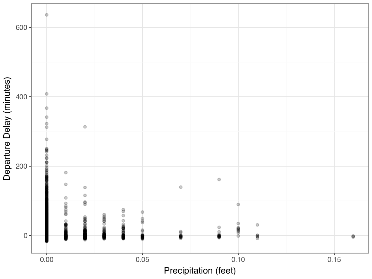
Hmmmm….where did all the data go?
How does rain affect departure delays?
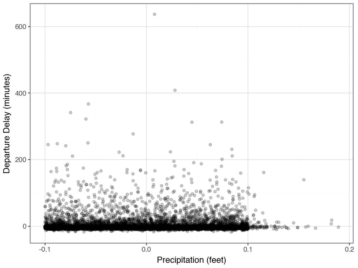
What changes would make this plot even better?
Joining on Keys with Different Names
Sometimes, the join keys have different names in the two data sets.
This frequently happens if the data sets come from different sources.
For example, suppose the airport was named
originindf_flightsbut was namedairportindf_weather.The
.merge()function providesleft_on =andright_on =arguments for specifying different column names in the left (first) and right (second) data sets.
Joining on Keys with Different Names
Joins with Missing Keys
Example: Baby names
The data below contains counts of names for babies born in 1920 and 2020:
1920
           Name Sex  Count
0          Mary   F  70975
1       Dorothy   F  36645
2         Helen   F  35098
3      Margaret   F  27997
4          Ruth   F  26100
...         ...  ..    ...
10751     Zearl   M      5
10752  Zeferino   M      5
10753      Zeke   M      5
10754      Zera   M      5
10755   Zygmont   M      5

[10756 rows x 3 columns]
2020
            Name Sex  Count
0         Olivia   F  17641
1           Emma   F  15656
2            Ava   F  13160
3      Charlotte   F  13065
4         Sophia   F  13036
...          ...  ..    ...
31448     Zykell   M      5
31449      Zylus   M      5
31450     Zymari   M      5
31451        Zyn   M      5
31452      Zyran   M      5

[31453 rows x 3 columns]
Joins
We can merge these two data sets on a their primary keys…
          Name Sex  Count_1920  Count_2020
0         Mary   F       70975        2210
1      Dorothy   F       36645         562
2        Helen   F       35098         721
3     Margaret   F       27997        2190
4         Ruth   F       26100        1323
...        ...  ..         ...         ...
4473     Whitt   M           5          23
4474     Wyley   M           5           6
4475    Xavier   M           5        3876
4476      York   M           5          14
4477      Zeke   M           5         382

[4478 rows x 4 columns]
What happened to some of the names?
Empty DataFrame
Columns: [Name, Sex, Count_1920, Count_2020]
Index: []Missing Keys
…but Maya is not in the 1920 data.
What type of join did the merge() function make by default?
An inner join!
Other Types of Joins
Types of Joins
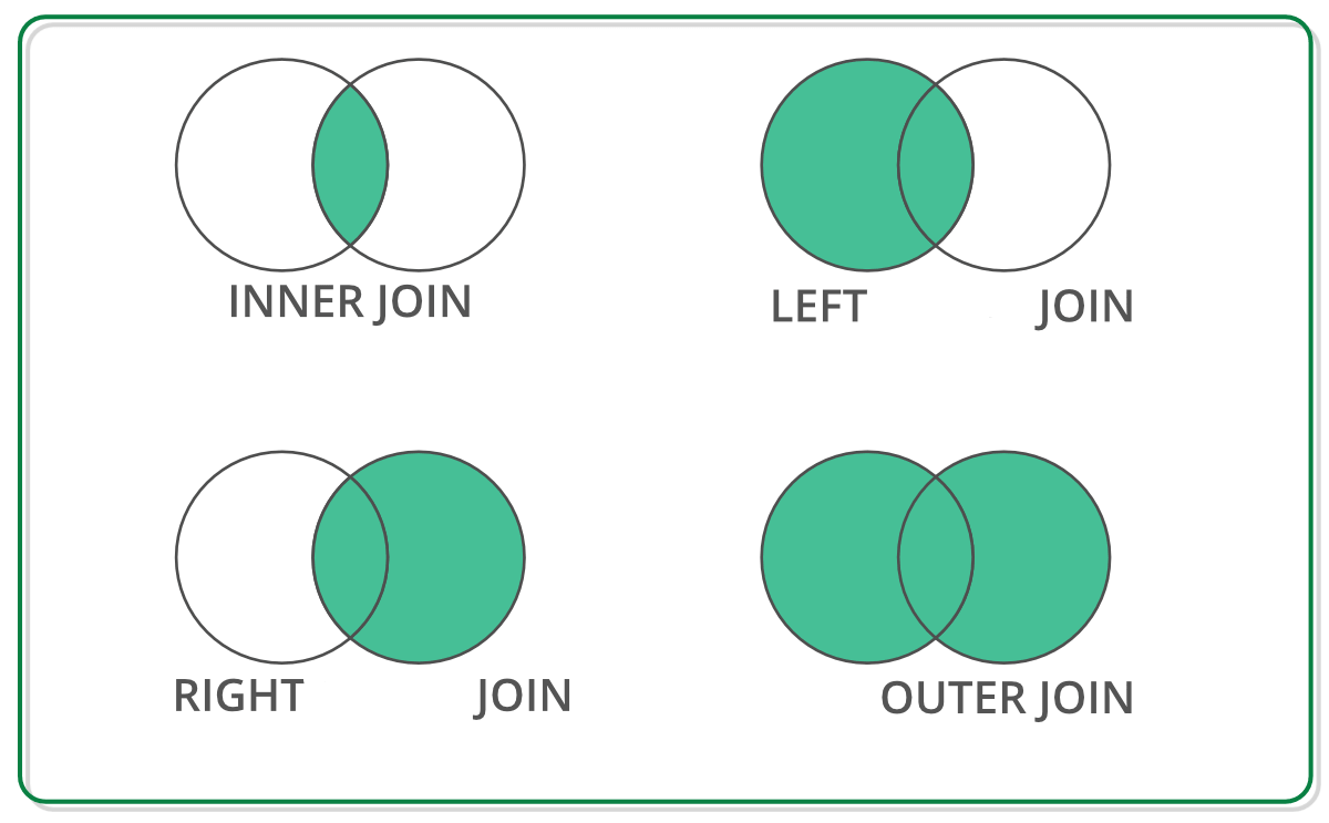
Types of Joins
We can customize the type of join using the how = parameter of .merge(). By default, how = "inner".
Types of Joins
Note the missing values for other columns, like
Count_1920!What other type of join would have produced this output in the Maya row?
Types of Joins
Note the missing values for other columns, like
Count_1920!What other type of join would have produced this output in the Maya row?
Quick Quiz
Which type of join would be best suited for each case?
- We want to determine the names that have increased in popularity the most between 1920 and 2020.
- We want to graph the popularity of names over time.
- We want to know what names from 1920 are no longer in use in 2020.
Filtering Joins
Filtering Joins
Inner, outer, left, and right are known as mutating joins, because they create new combined data sets.
There are two other types of joins that we use for filtering—to remove certain rows from the data.
Filtering Joins
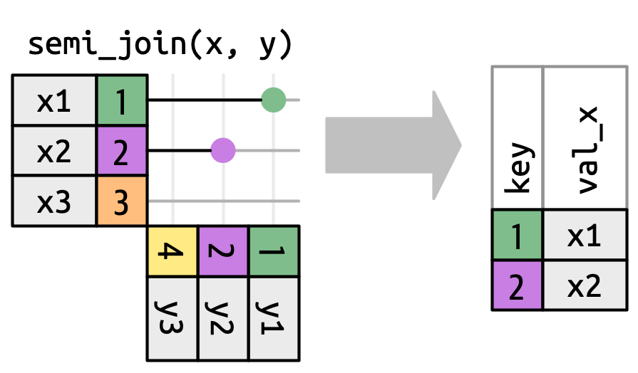
A semi-join tells us which keys in the left dataset are also present in the right dataset.
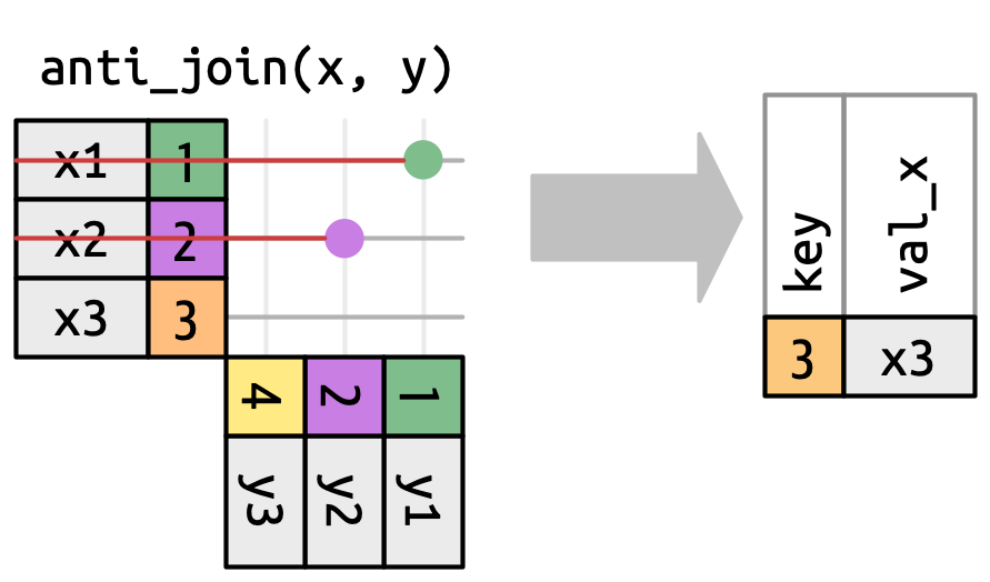
An anti-join tells us which keys in the left dataset are not present in the right dataset.
Filtering Joins
Which names existed in 1920 but don’t in 2020?
In Pandas, we can’t do these using .merge(), but we can use the isin() function!
Takeaways
Takeaways
A primary key is one or more columns that uniquely identify the rows.
We can join (a.k.a. merge) data sets if they share a primary key, or if one has a foreign key.
The default of
.merge()is an inner join: only keys in both data sets are kept.We can instead specify a left join, right join, or outer join; think about which rows we want to keep.
Filtering joins like anti-join and semi-join can help you answer questions about the data.
Use
.isin()to see which keys in one dataset exist in the other.