import pandas as pd

df = pd.read_csv("data/BreastTissue.csv")

cancer_levels = ["car", "fad", "mas"]
df['Cancerous'] = df['Class'].isin(cancer_levels)Logistic Regression
The story this week…
Classification
We can do KNN for Classification by letting the nearest neighbors “vote”.
The number of votes is a “probability”.
A classification model must be evaluated differently than a regression model.
One possible metric is accuracy, but this is a bad choice in situations with imbalanced data.
Precision measures “if we say it’s in Class A, is it really?”
Recall measures “if it’s really in Class A, did we find it?”
F1 Score is a balance of precision and recall.
Macro F1 Score averages the F1 scores of all classes.
What if there are ties?
In the last class a student (smartly) asked what would happen if there were ties.
- For example, if 2 of the 5 neighbors were from Group A, 2 were from Group B, and 1 was from Group C.
- The probabilities for Group A and Group B would be equal.
By default, KNeighborsClassifier() uses weights = "uniform", which selects the first occurrence of the maximum value. Meaning, the group that comes first in .classes_ is selected.
You can change this to prioritizing the group with the smallest distances by using weights = "distance".
Revisiting the Breast Cancer Data
Breast Tissue Classification
Electrical signals can be used to detect whether tissue is cancerous.
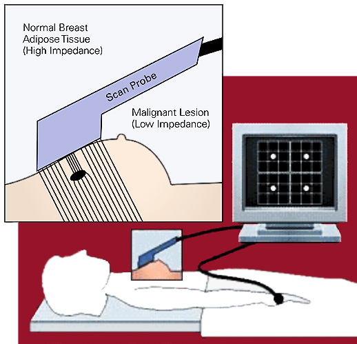
Analysis Goal
The goal is to determine whether a sample of breast tissue is:
Not Cancerous
- connective tissue
- adipose tissue
- glandular tissue
Cancerous
- carcinoma
- fibro-adenoma
- mastopathy
Binary response: Cancer or Not
Let’s read the data, and also make a new variable called “Cancerous”.
   Case # Class          I0  ...          DR           P  Cancerous
0       1   car  524.794072  ...  220.737212  556.828334       True
1       2   car  330.000000  ...   99.084964  400.225776       True
2       3   car  551.879287  ...  253.785300  656.769449       True
3       4   car  380.000000  ...  105.198568  493.701814       True
4       5   car  362.831266  ...  103.866552  424.796503       True

[5 rows x 12 columns]
Why not use “regular” regression?
You should NOT use ordinary regression for a classification problem!
This slide section is to show you why it does NOT work.
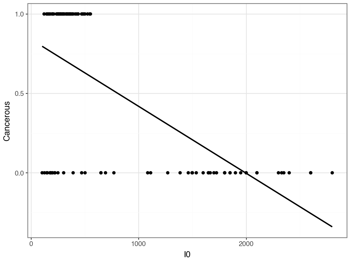
Counter-Example: Linear Regression
We know that in computers, True = 1 and False = 0. So, why not convert our response variable, Cancerous, to numbers and fit a regression?
   Case # Class          I0  ...          DR           P  Cancerous
0       1   car  524.794072  ...  220.737212  556.828334          1
1       2   car  330.000000  ...   99.084964  400.225776          1
2       3   car  551.879287  ...  253.785300  656.769449          1
3       4   car  380.000000  ...  105.198568  493.701814          1
4       5   car  362.831266  ...  103.866552  424.796503          1

[5 rows x 12 columns]
Counter-Example: Linear Regression
Counter-Example: Linear Regression
Problem 1: Did we get “reasonable” predictions?
Counter-Example: Linear Regression
Problem 2: How do we translate these predictions into categories???
array([ 0.74019045,  0.89022436,  0.82501565,  0.90210946,  0.82407215,
        0.70880368,  0.73084215,  0.75641256,  0.81285854,  0.84265773,
        1.05274916,  0.83203994,  0.82221736,  0.98879611,  0.84321428,
        1.14439789,  0.87065951,  0.82357191,  0.88721004,  0.86017708,
        0.75973787,  0.56958917,  0.50364921,  0.84044159,  0.66291026,
        0.5291845 ,  0.58770322,  0.58565156,  0.53944124,  0.54086431,
        0.626959  ,  0.60392716,  0.84459103,  0.65514535,  0.83767168,
        0.73230038,  0.82568408,  0.75333313,  0.54012942,  0.54183212,
        0.50716066,  0.70881584,  0.52734464,  0.66456375,  0.73629418,
        0.85237593,  0.84451578,  0.62061155,  0.60509501,  0.47440789,
        0.78797208,  0.74240828,  0.91841366,  0.71160435,  0.63338505,
        0.7122256 ,  0.82410488,  0.55742465,  0.62545421,  0.73912902,
        0.73912902,  0.70136245,  0.78113432,  0.77907358,  0.51597274,
        0.49247652,  0.65694204,  0.72574607,  0.76292245,  0.82501906,
        0.04266066,  0.24283615,  0.30785716,  0.52977377,  0.12835422,
        0.35012437,  0.39042852,  0.34447888,  0.10874534,  0.22844426,
        0.35125209,  0.25457208,  0.12820727,  0.18275452, -0.06826015,
       -0.02235371,  0.05662524, -0.02161184,  0.03275109, -0.03722977,
        0.05434446, -0.11400134,  0.0985149 , -0.01465065,  0.05067868,
        0.04211471,  0.05774736, -0.26666568, -0.13914904, -0.12585178,
       -0.02264956,  0.06060737,  0.04839979,  0.12583274, -0.17299232,
       -0.22474136])
Counter-Example: Linear Regression
Problem 3: Was the relationship really linear???
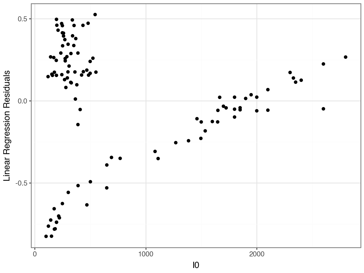
Counter-Example: Linear Regression
Problem 4: Are the errors really random???
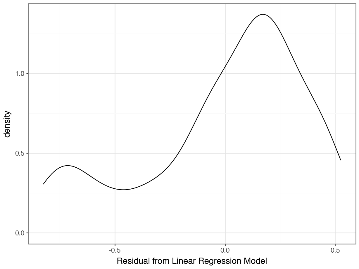
Counter-Example: Linear Regression
Problem 5: Are the errors normally distributed???
Logistic Regression
Logistic Regression
Idea: Instead of predicting 0 or 1, try to predict the probability of cancer.
Problem: We don’t observe probabilities before diagnosis; we only know if that person ended up with cancer or not.
Solution: (Fancy statistics and math.)
Why is it called Logistic Regression?
Because the “fancy math” uses a logistic function in it.
Logistic Regression
What you need to know:
It’s used for binary classification problems.
The predicted values are the “log-odds” of having cancer, i.e.
\[\text{log-odds} = \log \left(\frac{p}{1-p}\right)\]
We are more interested in the predicted probabilities.
As with KNN, we predict categories by choosing a threshold.
By default if \(p > 0.5\) -> we predict cancer
Logistic Regression in sklearn
No penalty
The "l2" penalty does ridge regression and is the default.
The "l1" penalty does lasso regression. Theelasticnet` penalty does lasso + ridge regression.
Logistic Regression in sklearn
array([1, 1, 1, 1, 1, 1, 1, 1, 1, 1, 1, 1, 1, 1, 1, 1, 1, 1, 1, 1, 1, 1,
       1, 1, 1, 1, 1, 1, 1, 1, 1, 1, 1, 1, 1, 1, 1, 1, 1, 1, 0, 1, 0, 1,
       1, 1, 1, 1, 1, 0, 1, 1, 1, 1, 1, 1, 1, 1, 1, 1, 1, 1, 1, 1, 0, 0,
       1, 1, 1, 1, 0, 0, 0, 0, 0, 0, 0, 0, 0, 0, 0, 0, 0, 0, 0, 0, 0, 0,
       0, 0, 0, 0, 0, 0, 0, 0, 0, 0, 0, 0, 0, 0, 0, 0, 0, 0])
Precison and Recall Revisited
Confusion Matrix
Code
    0   1
0  38  14
1   3  51
Calculate the precision for predicting cancer.
Calculate the recall for predicting cancer.
Calculate the precision for predicting non-cancer.
Calculate the recall for predicting non-cancer.
Threshold
What if we had used different cutoffs besides \(p > 0.5\)?
Higher Threshold
What we used \(p > 0.7\)?
Higher Threshold
What we used \(p > 0.7\)?
Code
    0   1
0  41  11
1 18 36Lower Threshold
What we used \(p > 0.2\)?
array([ True, True, True, True, True, True, True, True, True])Lower Threshold
    0   1
0  33  19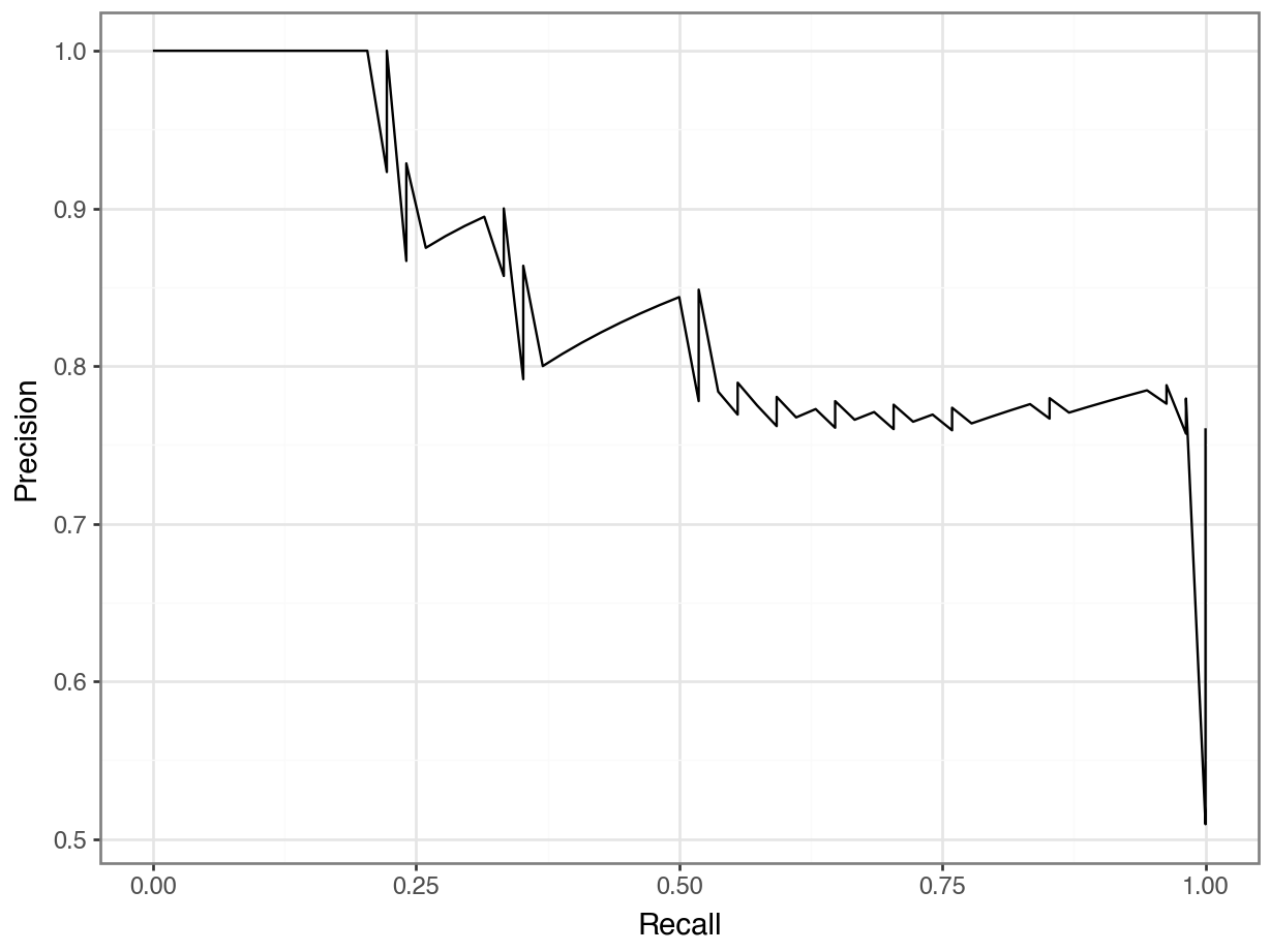
1 0 54Precision-Recall Curve
Precision-Recall Curve
Your turn
Activity
Suppose you want to predict Cancer vs. No Cancer from breast tissue using a Logistic Regression. Should you use…
Just
I0andPA500?Just
DAandP?I0,PA500,DA, andP?or all predictors?
Use cross-validation (cross_val_score()) with 10 folds using the F1 Score (scoring = "f1_macro") to decide!
Then, fit your final model and report the confusion matrix.
Interpreting Logistic Regression
Looking at Coefficients
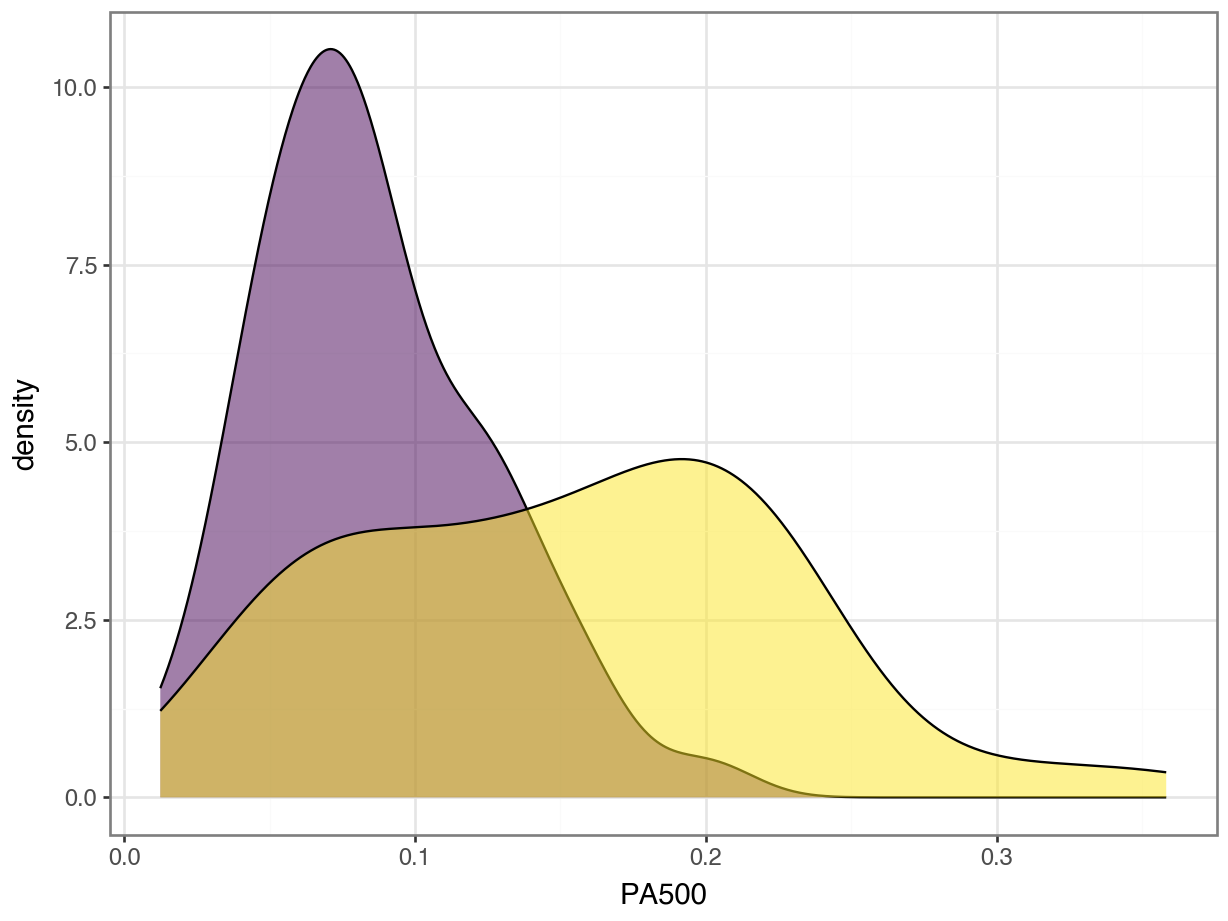
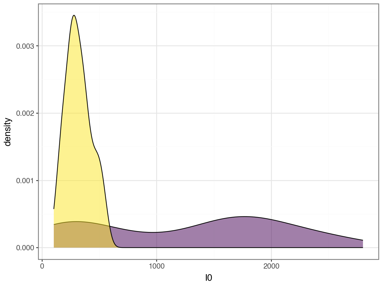
“For every unit of I0 higher, we predict 0.003 lower log-odds of cancer.”
“For every unit of PA500 higher, we predict 11.73 higher log-odds of cancer.”
Feature Importance
- Does this mean that
PA500is more important thanI0?
Standardization
Does this mean that
PA500is more important thanI0?Not necessarily. They have different units and so the coefficients mean different things.
“For every 1000 units of I0 higher, we predict 3.0 lower log-odds of cancer”
“For every 0.1 unit of PA500 higher, we predict 1.1 higher log-odds of cancer.”
What if we had standardized
I0andPA500?
Standardization
   Coefficients Column
0     -2.309090     I0
1      0.801477  PA500
Standardization
   Coefficients Column
0     -2.309090     I0
1 0.801477 PA500- “For every standard deviation above the mean someone’s
I0is, we predict 2.3 lower log-odds of cancer”
- “For every standard deviation above the mean someone’s
PA500is, we predict 0.80 higher log-odds of cancer.”
Standardization: Do you need it?
But - does this approach change our predictions?
   without_stdize  with_stdize
0        0.736188     0.736226
1        0.889803     0.889822
2        0.813277     0.813319
3        0.890781     0.890804
4        0.842957     0.842978
5        0.731660     0.731678
6        0.775454     0.775463
7        0.802116     0.802126
8        0.816982     0.817014
9        0.847675     0.847702
Standardization: Do you need it?
Standardizing will not change the predictions for Linear or Logistic Regression!
- This is because the coefficients are chosen relative to the units of the predictors. (Unlike in KNN!)
Advantage of not standardizing: More interpretable coefficients
- “For each unit of…” instead of “For each sd above the mean…”
Advantage of standardizing: Compare relative importance of predictors
It’s up to you!
- Don’t use cross-validation to decide - you’ll get the same metrics for both!
Your turn
Activity
For your Logistic Regression using all predictors, which variable was the most important?
How would you interpret the coefficient?
Takeaways
Takeaways
To fit a regression model (i.e., coefficients times predictors) to a categorical response, we use logistic regression.
Coefficients are interpreted as “One unit increase in predictor is associated with a [something] increase in the log-odds of Category 1.”
We still use cross-validated metrics to decide between KNN and Logistic regression, and between different feature sets.
We still report confusion matrices and sometimes precision-recall curves of our final model.