import pandas as pd
breast_df = pd.read_csv("data/BreastTissue.csv")Classification
Final Projects
Project Proposal - Due Sunday, February 23
The names of the members of your group.
Information about the dataset(s) you intend to analyze:
- Where are the data located?
- When were the data collected?
- Who collected the data?
- Why were the data collected?
- What information (variables) are in the dataset?
Research Questions: You should have one primary research question and a few secondary questions
Preliminary exploration of your dataset(s): A few simple plots or summary statistics that relate to the variables you plan to study.
The story so far…
Choosing a Best Model
We select a best model - aka best prediction procedure - by cross-validation.
Feature selection: Which predictors should we include, and how should we preprocess them?
Model selection: Should we use Linear Regression or KNN or Decision Trees or something else?
Hyperparameter tuning: Choosing model-specific settings, like \(k\) for KNN.
Each candidate is a pipeline; use
GridSearchCV()orcross_val_score()to score the options
Case Study: Breast Tissue Classification
Breast Tissue Classification
Electrical signals can be used to detect whether tissue is cancerous.
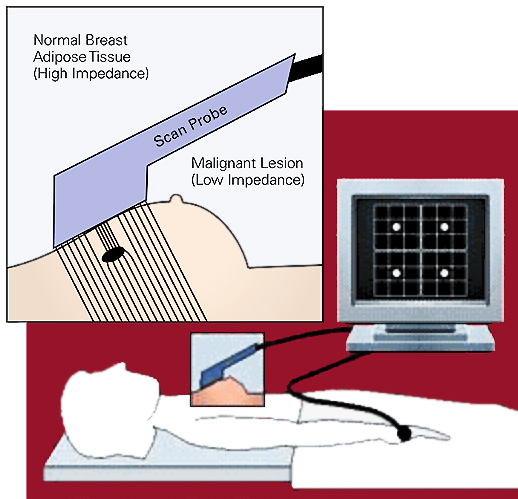
Analysis Goal
The goal is to determine whether a sample of breast tissue is:
Not Cancerous
- connective tissue
- adipose tissue
- glandular tissue
Cancerous
- carcinoma
- fibro-adenoma
- mastopathy
Reading in the Data
Case # Class I0 ... Max IP DR P
0 1 car 524.794072 ... 60.204880 220.737212 556.828334
1 2 car 330.000000 ... 69.717361 99.084964 400.225776
2 3 car 551.879287 ... 77.793297 253.785300 656.769449
3 4 car 380.000000 ... 88.758446 105.198568 493.701814
4 5 car 362.831266 ... 69.389389 103.866552 424.796503
.. ... ... ... ... ... ... ...
101 102 adi 2000.000000 ... 204.090347 478.517223 2088.648870
102 103 adi 2600.000000 ... 418.687286 977.552367 2664.583623
103 104 adi 1600.000000 ... 103.732704 432.129749 1475.371534
104 105 adi 2300.000000 ... 178.691742 49.593290 2480.592151
105 106 adi 2600.000000 ... 154.122604 729.368395 2545.419744
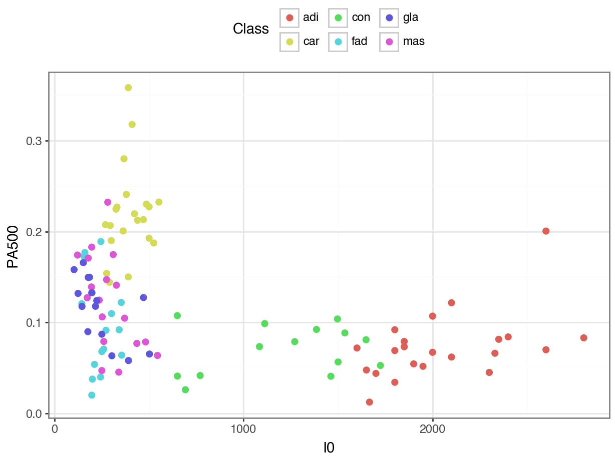
[106 rows x 11 columns]Variables of Interest
We will focus on two features:
- \(I_0\): impedivity at 0 kHz,
- \(PA_{500}\): phase angle at 500 kHz.
Visualizing the Data
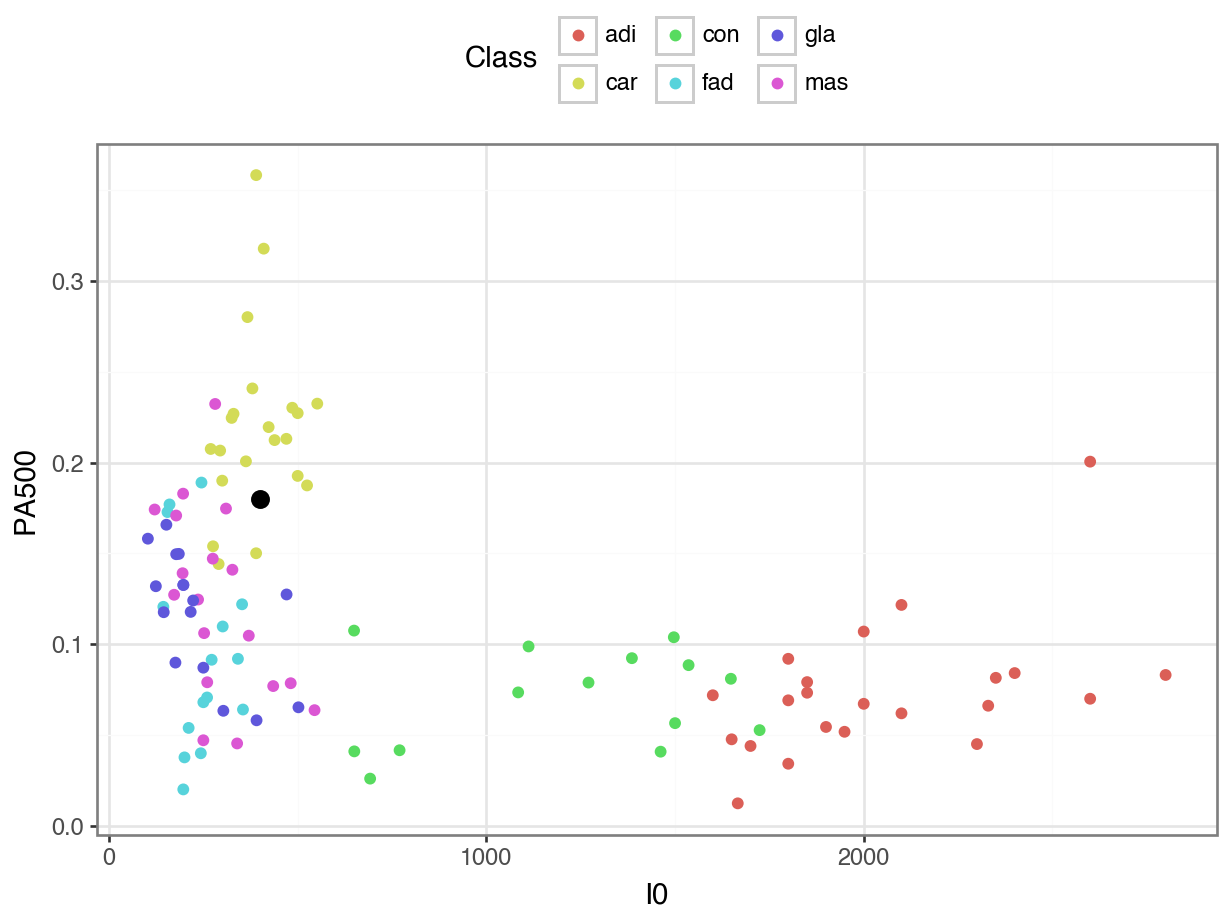
K-Nearest Neighbors Classification
K-Nearest Neighbors
What would we predict for someone with an \(I_0\) of 400 and a \(PA_{500}\) of 0.18?
K-Nearest Neighbors
Code
from plotnine import *

(
  ggplot() +
  geom_point(data = breast_df,
             mapping = aes(x = "I0", y = "PA500", color = "Class")) +
  geom_point(data = X_unknown,
             mapping = aes(x = "I0", y = "PA500"), size = 3) +
  theme_bw() +
  theme(legend_position = "top") +
  labs(x = "I0 (Impedivity at 0 kHz)",
       y = "Phase Angle at 500 kHz")
  )
K-Nearest Neighbors
This process is almost identical to KNN Regression:
Specify
Fit
Predict
Probabilities
Which of these two unknown points would we be more sure about in our guess?
Code
X_unknown = pd.DataFrame({"I0": [400, 2200], "PA500": [.18, 0.05]})

(
  ggplot() +
  geom_point(data = breast_df,
             mapping = aes(x = "I0", y = "PA500", color = "Class"),
             size = 2) +
  geom_point(data = X_unknown,
             mapping = aes(x = "I0", y = "PA500"), size = 3) +
  theme_bw() +
  theme(legend_position = "top") +
  labs(x = "I0 (Impedivity at 0 kHz)",
       y = "Phase Angle at 500 kHz")
    )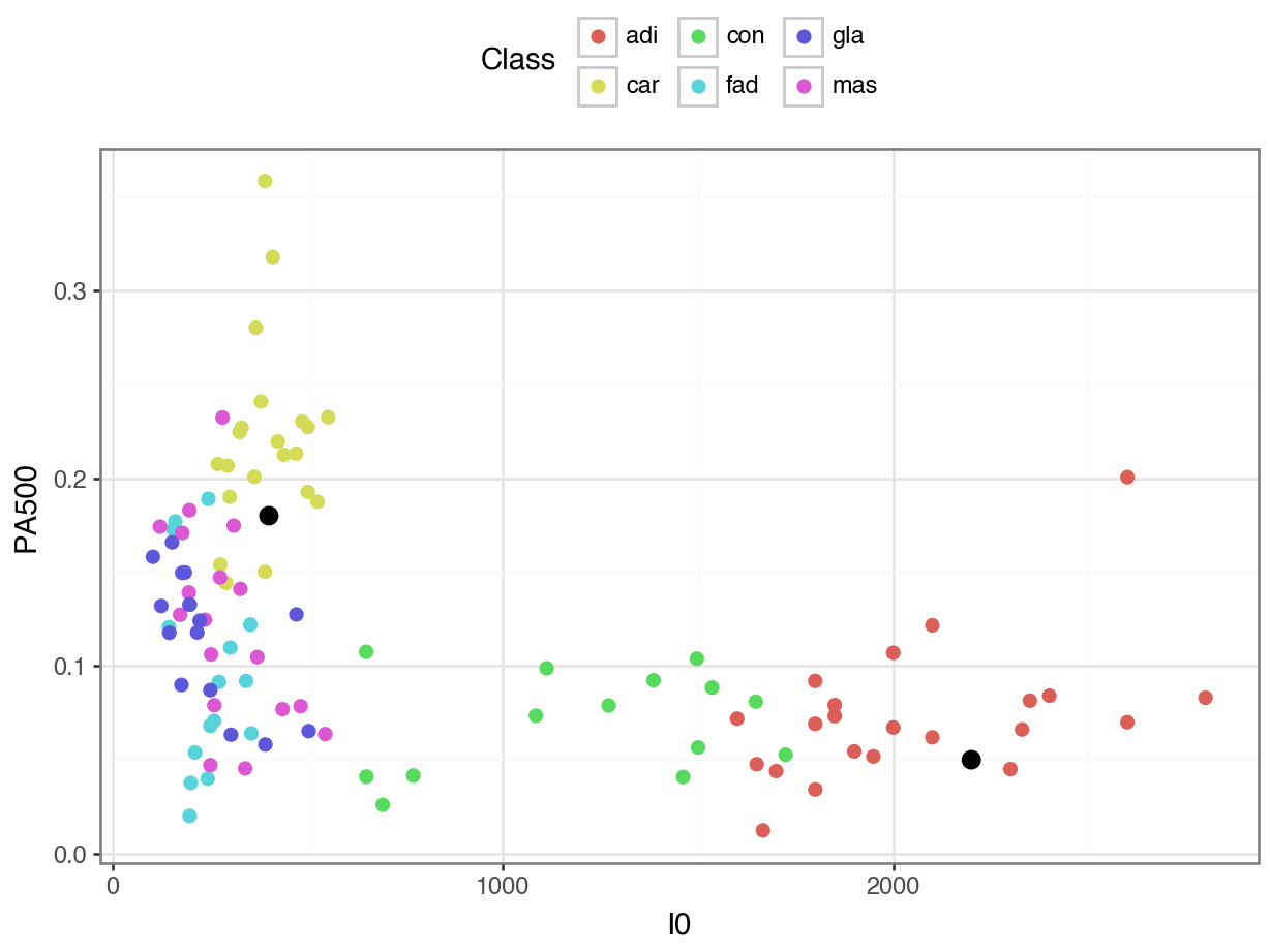
Probabilities
Instead of returning a single predicted class, we can ask sklearn to return the predicted probabilities for each class.
array([[0. , 0.6, 0. , 0.2, 0. , 0.2],
[1. , 0. , 0. , 0. , 0. , 0. ]])Tip
How did Scikit-Learn calculate these predicted probabilities?
Cross-Validation for Classification
We need a different scoring method for classification.
A simple scoring method is accuracy:
\[\text{accuracy} = \frac{\text{# correct predictions}}{\text{# predictions}}\]
Cross-Validation for Classification
Cross-Validation for Classification
As before, we can get an overall estimate of test accuracy by averaging the cross-validation accuracies:
But! Accuracy is not always the best measure of a classification model!
Confusion Matrix
Confusion Matrix with Classes
     adi  car  con  fad  gla  mas
adi   20    0    2    0    0    0
car    0   20    0    0    0    1
con    2    0   11    1    0    0
fad    0    0    0   13    1    1
gla    0    0    0    3   12    1
mas    0    2    0    8    3    5
What group(s) were the hardest to predict?
Activity
Activity
Use a grid search and the accuracy score to find the best k-value for this modeling problem.
Your grid should include:
- \(k\) (the number of neighbors)
- the distance metric (manhattan, euclidean)
- whether the mean should be used when standardizing
- whether the standard deviation should be used when standardizing
Classification Metrics
Case Study: Credit Card Fraud
            card4   card6 P_emaildomain  ...    C13    C14  isFraud
0            visa   debit     gmail.com  ...  637.0  114.0        0
1            visa   debit                ...    3.0    1.0        0
2            visa   debit     yahoo.com  ...    4.0    1.0        1
3            visa   debit   hotmail.com  ...    0.0    0.0        0
4            visa   debit     gmail.com  ...   20.0    1.0        0
...           ...     ...           ...  ...    ...    ...      ...
59049  mastercard   debit     gmail.com  ...    1.0    1.0        0
59050  mastercard  credit     yahoo.com  ...    1.0    1.0        0
59051  mastercard   debit    icloud.com  ...   15.0    2.0        0
59052        visa   debit     gmail.com  ...    1.0    1.0        1
59053  mastercard   debit                ...   84.0   17.0        0

[59054 rows x 19 columns]
Goal: Predict
isFraud, where 1 indicates a fraudulent transaction.
Classification Model
We can use \(k\)-nearest neighbors for classification:
from sklearn.preprocessing import OneHotEncoder
from sklearn.compose import make_column_transformer
from sklearn.compose import make_column_selector

ct = make_column_transformer(
    (StandardScaler(),
     make_column_selector(dtype_include = np.number)
     ),
    (OneHotEncoder(sparse_output = False),
     make_column_selector(dtype_include = object)
     ),
    remainder = "passthrough")

pipeline = make_pipeline(
  ct,
  KNeighborsClassifier(n_neighbors = 5)
  )
Training a Classifier
Isolating X and y for training data
How is the accuracy so high????
A Closer Look
Let’s take a closer look at the labels.
The vast majority of transactions aren’t fraudulent!
Imbalanced Data
If we just predicted that every transaction is normal, the accuracy would be \(1 - \frac{2119}{59054} = 0.964\) or 96.4%.
Even though such predictions would be accurate overall, it is inaccurate for fraudulent transactions.
A good model is “accurate for every class.”
Precision and Recall
We need a score that measures “accuracy for class \(c\)”!
There are at least two reasonable options:
Precision: \(P(\text{correct } | \text{ predicted class } c)\)
Among the observations that were predicted to be in class \(c\), what proportion actually were?
Recall: \(P(\text{correct } | \text{ actual class } c)\).
Among the observations that were actually in class \(c\), what proportion were predicted to be?
Precision and Recall by Hand
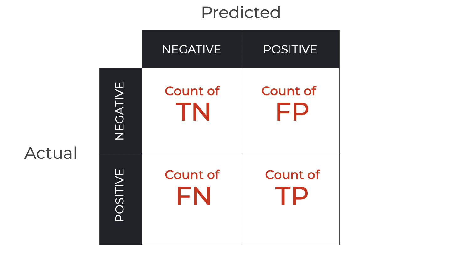
Precision is calculated as \(\frac{\text{TP}}{\text{TP} + \text{FP}}\).
Recall is calculated as \(\frac{\text{TP}}{\text{TP} + \text{FN}}\).
Precision and Recall by Hand
To check our understanding of these definitions, let’s calculate a few precisions and recalls by hand.
But first we need to get the confusion matrix!
Now Let’s Calculate!
What is the (training) accuracy?
What’s the precision for fraudulent transactions (
1)?What’s the recall for fraudulent transactions (
1)?
Trade Off Between Precision and Recall
Can you imagine a classifier that always has 100% recall for class \(c\), no matter the data?
In general, if the model classifies more observations as \(c\),
recall (for class \(c\)) \(\uparrow\)
precision (for class \(c\)) \(\downarrow\)
How do we compare two classifiers, if one has higher precision and the other has higher recall?
F1 Score
The F1 score combines precision and recall into a single score:
\[\text{F1 score} = \text{harmonic mean of precision and recall}\] \[= \frac{2} {\left( \frac{1}{\text{precision}} + \frac{1}{\text{recall}}\right)}\]
To achieve a high F1 score, both precision and recall have to be high.
If either is low, then the harmonic mean will be low.
Estimating Test Precision, Recall, and F1
Remember that each class has its own precision, recall, and F1.
But Scikit-Learn requires that the
scoringparameter be a single metric.For this, we can average the score over the metrics:
"precision_macro""recall_macro""f1_macro"
F1 Score
Precision-Recall Curve
Another way to illustrate the trade off between precision and recall is to graph the precision-recall curve.
First, we need the predicted probabilities.
Precision-Recall Curve
By default, Scikit-Learn classifies a transaction as fraud if this probability is \(> 0.5\).
What if we instead used a threshold
tother than \(0.5\)?Depending on which
twe pick, we’ll get a different precision and recall.
We can graph this trade off!
Precision-Recall Curve
Let’s graph the precision-recall curve together in a Colab.
https://colab.research.google.com/drive/1T-0iQOQZFldHNmOXdZf4GU0b8j3kWMc_?usp=sharing
Takeaways
Takeaways
We can do KNN for Classification by letting the nearest neighbors “vote”
The number of votes is a “probability”
A classification model must be evaluated differently than a regression model.
One possible metric is accuracy, but this is a bad choice in situations with imbalanced data.
Precision measures “if we say it’s in Class A, is it really?”
Recall measures “if it’s really in Class A, did we find it?”
F1 Score is a balance of precision and recall
Macro F1 Score averages the F1 scores of all classes