Cross-Validation and Grid Search
Final Project Groups
Let’s take 5-minutes and form groups with other students in the class!
Reporting Your Group
Did you find a group to work with? Please fill out this form!
Do you still need to find a group to work with? Please fill out this form!
Exam 1
Revision Opportunities
You have the opportunity to earn back up to 75% of the points you lost.
Revisions must include reflections addressing:
- what aspects of your previous answer were incorrect / misleading / incomplete
- what you changed about your answer to remedy this issue
- what you learned during this process
Revisions are about learning
As such, your reflections should tell me (briefly) what you learned. Quality of reflection is better than quantity.
Revision Submissions - Due Monday, February 23 at 5pm
Revisions should be done in a new (clean) Colab Notebook
- Reflections should come at the beginning of each problem
Your revisions will be submitted to the same assignment portal
To be eligible for regrading, your revisions must be:
- Submitted as a PDF (with a Colab link)
- Printed to landscape
- Have all your code visible
- Reflections for every problem being revised
The story so far…
Modeling
We assume some process \(f\) is generating our target variable:
target = f(predictors) + noise
Our goal is to come up with an approximation of \(f\).
Test Error vs Training Error
We don’t need to know how well our model does on training data.
We want to know how well it will do on test data.
In general, test error \(>\) training error.
Analogy: A professor posts a practice exam before an exam.
If the actual exam is the same as the practice exam, how many points will students miss? That’s training error.
If the actual exam is different from the practice exam, how many points will students miss? That’s test error.
It’s always easier to answer questions that you’ve seen before than questions you haven’t seen.
Modeling Procedure
For each model proposed:
Establish a pipeline with transformers and a model.
Fit the pipeline on the training data (with known outcome)
Predict with the fitted pipeline on test data (with known outcome)
Evaluate our success; i.e., measure noise “left over”
Then:
Select the best model
Fit on all the data
Predict on any future data (with unknown outcome)
Linear Regression
Simple Linear Model
We assume that the target (\(Y\)) is generated from an equation of the predictor (\(X\)), plus random noise (\(\epsilon\))
\[Y = \beta_0 + \beta_1 X + \epsilon\]
Goal: Use observations \((x_1, y_1), ..., (x_n, y_n)\) to estimate \(\beta_0\) and \(\beta_1\).
What are these parameters???
In Statistics, we use \(\beta_0\) to represent the population intercept and \(\beta_1\) to represent the slope. By “population” we mean the true slope of the line for the entire population of interest.
Measures of Success
What is the “best” choice of \(\widehat{\beta}_0\) and \(\widehat{\beta}_1\) (the estimates of \(\beta_0\) and \(\beta_1\))?
The ones that are statistically most justified, under certain assumptions about \(Y\) and \(X\)?
The ones that are “closest to” the observed points?
- \(|\widehat{y}_i - y_i|\)?
- \((\widehat{y}_i - y_i)^2\)?
- \((\widehat{y}_i - y_i)^4\)?
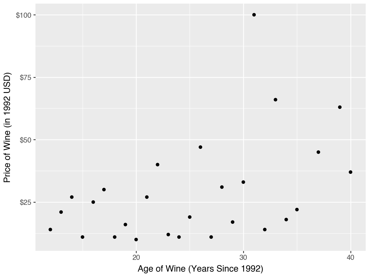
Example: Wine Data
Price Predicted by Age of Wine
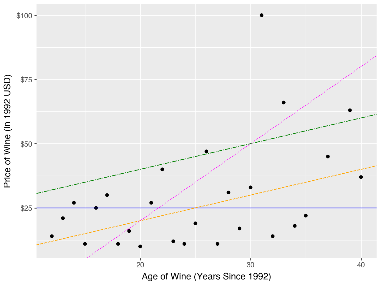
“Candidate” Regression Lines
Consider five possible regression equations:
\[\text{price} = 25 + 0*\text{age}\] \[\text{price} = 0 + 1*\text{age}\] \[\text{price} = 20 + 1*\text{age}\] \[\text{price} = -40 + 3*\text{age}\]
Which one do you think will be “closest” to the points on the scatterplot?
“Candidate” Regression Lines
Code
(
  ggplot(data = df_known, mapping = aes(x = "age", y = "price")) +
  geom_point() +
  labs(x = "Age of Wine (Years Since 1992)",
       y = "Price of Wine (in 1992 USD)") +
  scale_y_continuous(labels = currency_format(precision = 0)) +
  geom_abline(intercept = 25,
              slope = 0,
              color = "blue",
              linetype = "solid") +
  geom_abline(intercept = 0,
              slope = 1,
              color = "orange",
              linetype = "dashed") +
  geom_abline(intercept = 20,
              slope = 1,
              color = "green") +
  geom_abline(intercept = -40,
              slope = 3,
              color = "magenta")
  )
The “best” slope and intercept
It’s clear that some of these lines are better than others.
How to choose the best? Math!
We’ll let the computer do it for us.
Caution
The estimated slope and intercept are calculated from the training data at the .fit() step.
Linear Regression in sklearn
Specify
Fit
Pipeline(steps=[('linearregression', LinearRegression())])In a Jupyter environment, please rerun this cell to show the HTML representation or trust the notebook. On GitHub, the HTML representation is unable to render, please try loading this page with nbviewer.org.
Parameters
Parameters
Estimated Intercept and Slope
Fitting and Predicting
To predict from a linear regression, we just plug in the values to the equation…
Fitting and Predicting with .predict()
To predict from a linear regression, we just plug in the values to the equation…
Questions to ask yourself
Q: Is there only one “best” regression line?
A: No, you can justify many choices of slope and intercept! But there is a generally accepted approach called Least Squares Regression that we will always use.
Q: How do you know which variables to include in the equation?
A: Try them all, and see what predicts best.
Q: How do you know whether to use linear regression or KNN to predict?
A: Try them both, and see what predicts best!
Cross-Validation
Resampling methods
We saw that a “fair” way to evaluate models was to randomly split into training and test sets.
But what if this randomness was misleading? (e.g., a major outlier in one of the sets)
What do we usually do in Statistics to address randomness? Take many samples and compute an average!
A resampling method is when we take many random test / training splits and average the resulting metrics.
Resampling Method Example
Import all our functions:
Creating Testing & Training Splits
- This creates four new objects,
X_train,X_test,y_train, andy_test.- Note that the objects are created in this order!
- The “testing” data are 10% (0.1) of the total size of the training data (
df_known).
Pipeline for Predicting on Test Data
Specify
Fit for Training Data
Predict for Test Data
Estimating Error for Test Data
Cross-Validation
It makes sense to do test / training many times…
But! Remember the original reason for test / training: we don’t want to use the same data in fitting and evaluation.
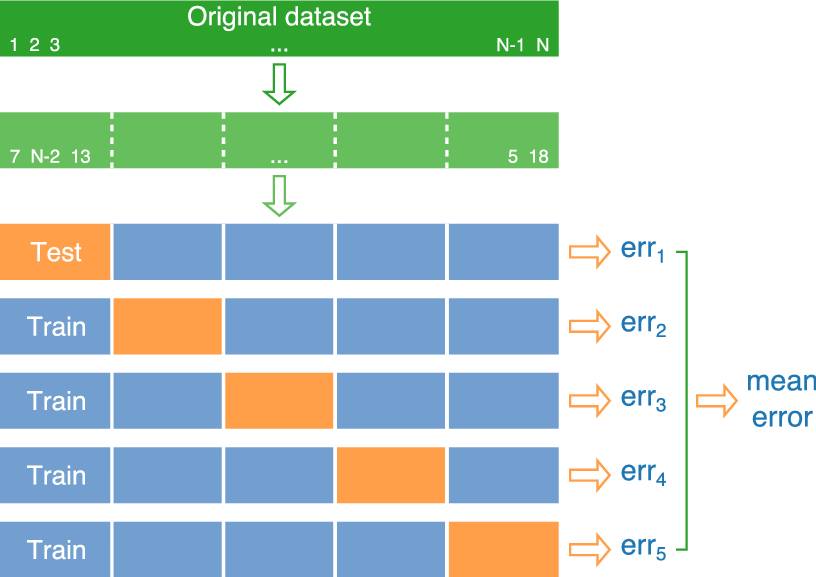
Idea: Let’s make sure that each observation only gets to be in the test set once
- Cross-validation: Divide the data into 10 random “folds”. Each fold gets a “turn” as the test set.
Cross-Validation (5-Fold)
Cross-Validation in sklearn
Cross-Validation in sklearn
What are these numbers?
sklearnchooses a default metric for you based on the model.In the case of regression, the default metric is R-Squared.
The metrics from sklearn will always want to be maximized.
- Larger R-Squared values explain more of the variance in the response (y).
- Larger negative RMSE (smaller RMSE) means the “leftover” variance in y is minimized.
What do we do with these numbers?
Since we have 10 different values, what would you expect us to do?
Cross-Validation in sklearn
What if you want MSE?
Cross-Validation: FAQ
Q: How many cross validations should we do?
A: It doesn’t matter much! Typical choices are 5 or 10.
A: Think about the trade-offs:
- larger training sets = more accurate models
- smaller test sets = more uncertainty in evaluation
Q: What metric should we use?
A: This is also your choice! What captures your idea of a “successful prediction”? MSE / RMSE is a good default, but you might find other options that are better!
Q: I took a statistics class before, and I remember some things like “adjusted R-Squared” or “AIC” for model selection. What about those?
A: Those are Old School, from a time when computers were not powerful enough to do cross-validation. Modern data science uses resampling!
Activity
Your turn
Use cross-validation to choose between Linear Regression and KNN with k = 7 based on
"neg_mean_squared_error", for:- Using all predictors.
- Using just winter rainfall and summer temperature.
- Using only age.
Re-run #1, but instead use mean absolute error. (You will need to look in the documentation of
cross_val_score()for this!)
Tuning with GridSearchCV()
Tuning
In previous classes, we tried many different values of \(k\) for KNN.
We also mentioned using absolute distance (Manhattan) instead of euclidean distance.
Now, we would like to use cross-validation to decide between these options.
sklearn provides a nice shortcut for this!
Initializing GridSearchCV()
Fitting GridSearchCV()
GridSearchCV(cv=5,
             estimator=Pipeline(steps=[('columntransformer',
                                        ColumnTransformer(transformers=[('standardscaler',
                                                                         StandardScaler(),
                                                                         ['summer',
                                                                          'har',
                                                                          'sep',
                                                                          'win',
                                                                          'age'])])),
                                       ('kneighborsregressor',
                                        KNeighborsRegressor())]),
             param_grid={'kneighborsregressor__metric': ['euclidean',
                                                         'manhattan'],
                         'kneighborsregressor__n_neighbors': range(1, 7)},
             scoring='neg_mean_squared_error')
In a Jupyter environment, please rerun this cell to show the HTML representation or trust the notebook. On GitHub, the HTML representation is unable to render, please try loading this page with nbviewer.org.
Parameters
Parameters
['summer', 'har', 'sep', 'win', 'age']
Parameters
Parameters
How many different models were fit with this grid?
Getting the Cross Validation Results
    mean_fit_time  std_fit_time  ...  std_test_score  rank_test_score
0        0.001124      0.000289  ...      219.338831               12
1        0.000961      0.000018  ...      209.511631                9
2        0.000955      0.000018  ...      178.819362                6
3        0.000956      0.000018  ...      217.989122               11
4        0.000953      0.000020  ...      212.797774                7
5        0.000946      0.000008  ...      205.240907                3
6        0.000952      0.000017  ...      227.978005               10
7        0.000950      0.000021  ...      175.175403                2
8        0.001004      0.000127  ...      174.981203                5
9        0.000925      0.000015  ...      175.186322                1
10       0.000941      0.000017  ...      200.091917                4
11       0.000933      0.000008  ...      232.710455                8

[12 rows x 15 columns]
What about k and the distances?
   param_kneighborsregressor__metric  ...  mean_test_score
0                          euclidean  ...      -321.833333
1                          euclidean  ...      -292.281667
2                          euclidean  ...      -278.301481
3                          euclidean  ...      -308.950417
4                          euclidean  ...      -279.847733
5                          euclidean  ...      -259.804074
6                          manhattan  ...      -305.793333
7                          manhattan  ...      -254.886667
8                          manhattan  ...      -274.401481
9                          manhattan  ...      -232.973333
10                         manhattan  ...      -267.988800
11                         manhattan  ...      -282.869444

[12 rows x 3 columns]
What were the best parameters?
Model Evaluation
You have now encountered three types of decisions for finding your best model:
Which predictors should we include, and how should we preprocess them? (Feature selection)
Should we use Linear Regression or KNN or something else? (Model selection)
Which value of \(k\) should we use? (Parameter tuning)
Model Evaluation
Think of this like a college sports bracket:
Gather all your candidate pipelines (combinations of column transformers and model specifications)
Tune each pipeline with cross-validation (regional championships!)
Determine the best model type for each feature set (state championships!)
Determine the best pipeline (national championships!)