K-Nearest-Neighbors

Exam 1 Reminders

What to expect

Content

Everything covered through the end of this week
- Visualizing numerical & categorical variables
- Summarizing numerical & categorical variables
- Distances between observations
- Preprocessing (scaling / one-hot-encoding) variables

Structure

80-minutes
- First part of class (8:10 - 9:30am; 12:10 - 1:30pm)
Google Collab Notebook
Resources you can use:
- Your own Collab notebooks
- Any course materials
- Official Python documentation
Resources you can not use:
- Other humans
- Generative AI for anything beyond text completion
- Google for anything except to reach Python documentation pages

A Reminder about Code Complexity

There are always multiple ways to accomplish a given task.

In addition to accomplishing the given task, your grade on each problem will also depend on:

whether your solution uses tools taught in this class, and
the efficiency of your solution (e.g., did you use a for loop when it was not necessary?)

Efficiency in Preprocessing

all_transformer = make_column_transformer(
    (StandardScaler(),
     ["abv", "srm", "originalGravity", "ibu"]
     ),
    (OneHotEncoder(sparse_output = False),
     ["isOrganic", "glass", "available"]
     ),
    remainder = "drop")

all_transformer = make_column_transformer(
    (StandardScaler(),
     make_column_selector(dtype_include = np.number)
     ),
    (OneHotEncoder(sparse_output = False),
     make_column_selector(dtype_include = object)
     ),
    remainder = "drop")

What are the efficiency benefits of making a general preprocessor?

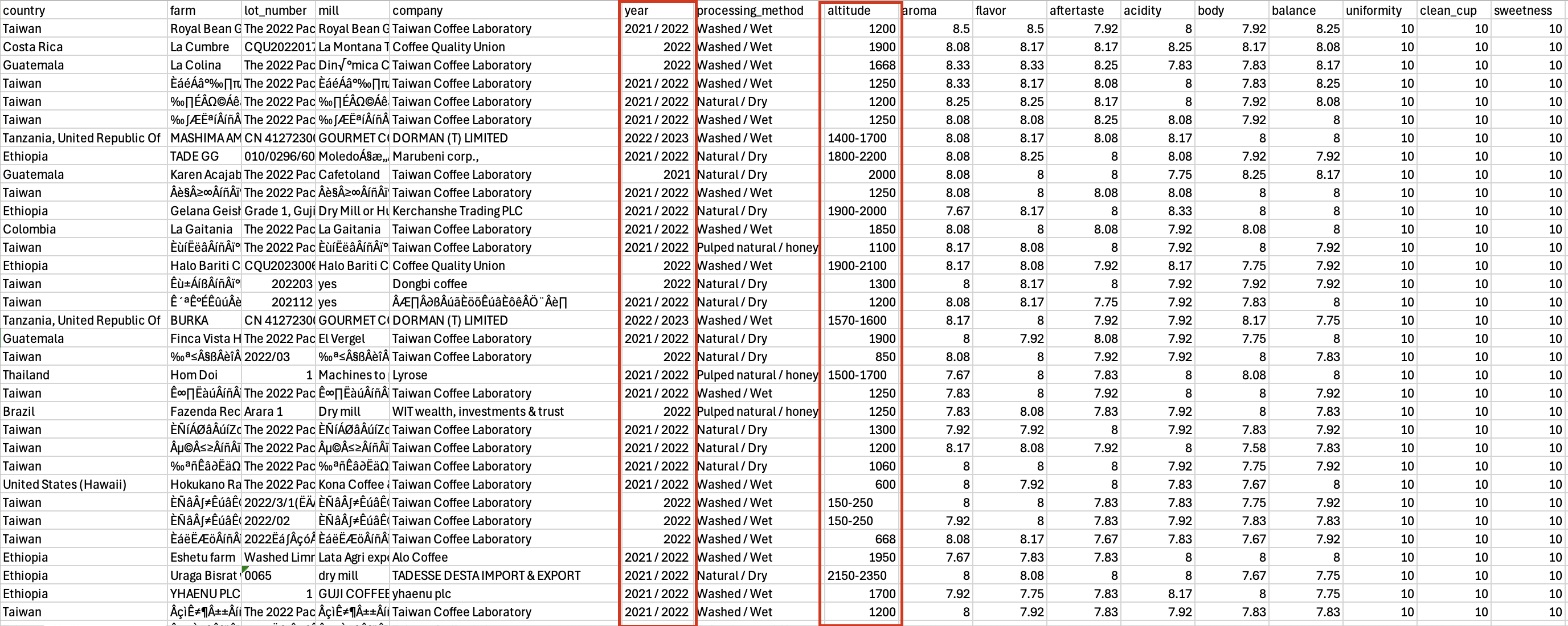
Data for Exam 1

Your analysis will focus on the qualitites of different types of coffee and how they are related to where / when / how the coffee was grown and processed.

A screenshot of the `coffee.csv` data file you will be analyzing for your Midterm Exam. The preview shows 17 different columns, with two columns highlighted in red---year and altitude. These columns are highlighted because they contain values with some inconsistent formats and may be needed to be cleaned before analysis. — Link to the raw data)

The story so far…

Steps for data analysis

Read and then clean the data
- Are there missing values? Will we drop those rows, or replace the missing values with something?
- Are there quantitative variables that Python thinks are categorical?
- Are there categorical variables that Python thinks are quantitative?
- Are there any anomalies in the data that concern you?

Steps for data analysis (cont’d)

Explore the data by visualizing and summarizing.
- Different approaches for different combos of quantitative and categorical variables.
- Think about conditional calculations (split-apply-combine)

Steps for data analysis (cont’d)

Identify a research question of interest.
Perform preprocessing steps
- Should we scale the quantitative variables?
- Should we one-hot-encode the categorical variables?
- Should we log-transform any variables?
Measure similarity between observations by calculating distances.
- Which features should be included?
- Which distance metric should we use?

Predicting Wine Prices

Data: Wine Qualities

df = pd.read_csv("https://dlsun.github.io/pods/data/bordeaux.csv")
df

    year  price  summer  har   sep  win  age
0   1952   37.0    17.1  160  14.3  600   40
1   1953   63.0    16.7   80  17.3  690   39
2   1955   45.0    17.1  130  16.8  502   37
3   1957   22.0    16.1  110  16.2  420   35
4   1958   18.0    16.4  187  19.1  582   34
5   1959   66.0    17.5  187  18.7  485   33
6   1960   14.0    16.4  290  15.8  763   32
7   1961  100.0    17.3   38  20.4  830   31
8   1962   33.0    16.3   52  17.2  697   30
9   1963   17.0    15.7  155  16.2  608   29
10  1964   31.0    17.3   96  18.8  402   28
11  1965   11.0    15.4  267  14.8  602   27
12  1966   47.0    16.5   86  18.4  819   26
13  1967   19.0    16.2  118  16.5  714   25
14  1968   11.0    16.2  292  16.4  610   24
15  1969   12.0    16.5  244  16.6  575   23
16  1970   40.0    16.7   89  18.0  622   22
17  1971   27.0    16.8  112  16.9  551   21
18  1972   10.0    15.0  158  14.6  536   20
19  1973   16.0    17.1  123  17.9  376   19
20  1974   11.0    16.3  184  16.2  574   18
21  1975   30.0    16.9  171  17.2  572   17
22  1976   25.0    17.6  247  16.1  418   16
23  1977   11.0    15.6   87  16.8  821   15
24  1978   27.0    15.8   51  17.4  763   14
25  1979   21.0    16.2  122  17.3  717   13
26  1980   14.0    16.0   74  18.4  578   12
27  1981    NaN    17.0  111  18.0  535   11
28  1982    NaN    17.4  162  18.5  712   10
29  1983    NaN    17.4  119  17.9  845    9
30  1984    NaN    16.5  119  16.0  591    8
31  1985    NaN    16.8   38  18.9  744    7
32  1986    NaN    16.3  171  17.5  563    6
33  1987    NaN    17.0  115  18.9  452    5
34  1988    NaN    17.1   59  16.8  808    4
35  1989    NaN    18.6   82  18.4  443    3
36  1990    NaN    18.7   80  19.3  468    2
37  1991    NaN    17.7  183  20.4  570    1

Data: Wine Quality Variables

year: What year the wine was produced
price: Average market price for Bordeaux vintages according to a series of auctions.
- The price is relative to the price of the 1961 vintage, regarded as the best one ever recorded.
win: Winter rainfall (in mm)
summer: Average temperature during the summer months (June - August)
sep: Average temperature in the month of September (in Celsius)
har: Rainfall during harvest month(s) (in mm)
age: How old the wine was in 1992 (years since 1992)

Analysis Goal

Goal: Predict what will be the quality (price) of wines in a future year.

Idea: Wines with similar features probably have similar quality.

Inputs: Summer temperature, harvest rainfall, September temperature, winter rainfall, age of wine
- “Inputs” = “Features” = “Predictors” = “Independent variables”
Output: Price in 1992
- “Output” = “Target” = “Dependent variable”

Similar Wines

Which wines have similar summer temps and winter rainfall to the 1989 vintage?

Code

from plotnine import *

(
  ggplot(df, mapping = aes(x = "summer", y = "win")) + 
  geom_point(color = "white") + 
  geom_text(mapping = aes(label = "year")) + 
  theme_bw()
)

Predicting 1989

1989

df[df['year'] == 1989]

    year  price  summer  har   sep  win  age
35  1989    NaN    18.6   82  18.4  443    3

1990

df[df['year'] == 1990]

    year  price  summer  har   sep  win  age
36  1990    NaN    18.7   80  19.3  468    2

1976

df[df['year'] == 1976]

    year  price  summer  har   sep  win  age
22  1976   25.0    17.6  247  16.1  418   16

Training and test data

The data for which we know the target is called the training data.

known_prices = df['year'] < 1981

df_train = df[known_prices].copy()

The data for which we don’t know the target (and want to predict it) is called the test data.

to_predict = df['year'] == 1989

df_test = df[to_predict].copy()

Testing & Training with `scikitlearn`

Specify steps

First we make a column transformer…

from sklearn.compose import make_column_transformer
from sklearn.compose import make_column_selector
from sklearn.preprocessing import OneHotEncoder
from sklearn.preprocessing import StandardScaler

preproc = make_column_transformer(
  (StandardScaler(), 
  make_column_selector(dtype_include = np.number)
  ),
  remainder = "drop"
)

features = ['summer', 'har', 'sep', 'win', 'age']

Why make a general processor?

Fit the Preprocesser

Then we fit it on the training data.

preproc.fit(df_train[features])

ColumnTransformer(transformers=[('standardscaler', StandardScaler(),
                                 <sklearn.compose._column_transformer.make_column_selector object at 0x119f95c90>)])

In a Jupyter environment, please rerun this cell to show the HTML representation or trust the notebook.
On GitHub, the HTML representation is unable to render, please try loading this page with nbviewer.org.

preproc.named_transformers_['standardscaler'].mean_

array([ 16.47037037, 144.81481481,  17.04814815, 608.40740741,
        25.18518519])

preproc.named_transformers_['standardscaler'].var_

array([4.09492455e-01, 5.14089163e+03, 1.89286694e+00, 1.60333525e+04,
       6.54842250e+01])

Prep the data

Then we transform the training data AND the test data:

train_new = preproc.transform(df_train[features])
test_new = preproc.transform(df_test[features])

test_new

array([[ 3.32798322, -0.87607817,  0.98258257, -1.30629957, -2.74154079]])

What if we had fit on the test data?

preproc.fit(df_test[features])

ColumnTransformer(transformers=[('standardscaler', StandardScaler(),
                                 <sklearn.compose._column_transformer.make_column_selector object at 0x119f95c90>)])

preproc.named_transformers_['standardscaler'].mean_

array([ 18.6,  82. ,  18.4, 443. ,   3. ])

preproc.named_transformers_['standardscaler'].var_

array([0., 0., 0., 0., 0.])

What if we had fit on the test data?

preproc.transform(df_test[features])

array([[0., 0., 0., 0., 0.]])

All together:

preproc = make_column_transformer(
  (StandardScaler(), 
  make_column_selector(dtype_include = np.number)
  ),
  remainder = "drop"
)

features = ['summer', 'har', 'sep', 'win', 'age']

preproc.fit(df_train[features])

ColumnTransformer(transformers=[('standardscaler', StandardScaler(),
                                 <sklearn.compose._column_transformer.make_column_selector object at 0x119f96fb0>)])

train_new = preproc.transform(df_train[features])
test_new = preproc.transform(df_test[features])

Find the Closest k

from sklearn.metrics import pairwise_distances

dists = pairwise_distances(test_new, train_new)
dists

array([[6.16457005, 5.74908409, 5.01651675, 5.8002254 , 5.48664619,
        4.35898872, 6.56017889, 5.28491106, 5.38614546, 6.01267804,
        3.72811494, 6.99167472, 5.26008007, 5.3100901 , 5.76468136,
        4.97806644, 4.05228644, 3.86667994, 6.7345252 , 3.18480532,
        4.69099623, 3.65924   , 3.62660714, 5.86910657, 5.30050409,
        4.60719435, 4.34675994]])

Find the Closest k

best = (
  dists[0]
  .argsort()
  )
best[0:5]

array([19, 22, 21, 10, 17])

df_train.loc[best]

    year  price  summer  har   sep  win  age
19  1973   16.0    17.1  123  17.9  376   19
22  1976   25.0    17.6  247  16.1  418   16
21  1975   30.0    16.9  171  17.2  572   17
10  1964   31.0    17.3   96  18.8  402   28
17  1971   27.0    16.8  112  16.9  551   21
16  1970   40.0    16.7   89  18.0  622   22
26  1980   14.0    16.0   74  18.4  578   12
5   1959   66.0    17.5  187  18.7  485   33
25  1979   21.0    16.2  122  17.3  717   13
20  1974   11.0    16.3  184  16.2  574   18
15  1969   12.0    16.5  244  16.6  575   23
2   1955   45.0    17.1  130  16.8  502   37
12  1966   47.0    16.5   86  18.4  819   26
7   1961  100.0    17.3   38  20.4  830   31
24  1978   27.0    15.8   51  17.4  763   14
13  1967   19.0    16.2  118  16.5  714   25
8   1962   33.0    16.3   52  17.2  697   30
4   1958   18.0    16.4  187  19.1  582   34
1   1953   63.0    16.7   80  17.3  690   39
14  1968   11.0    16.2  292  16.4  610   24
3   1957   22.0    16.1  110  16.2  420   35
23  1977   11.0    15.6   87  16.8  821   15
9   1963   17.0    15.7  155  16.2  608   29
0   1952   37.0    17.1  160  14.3  600   40
6   1960   14.0    16.4  290  15.8  763   32
18  1972   10.0    15.0  158  14.6  536   20
11  1965   11.0    15.4  267  14.8  602   27

Predict from the closest k

If \(k = 1\) …

df_train.loc[best[0]]

year      1973.0
price       16.0
summer      17.1
har        123.0
sep         17.9
win        376.0
age         19.0
Name: 19, dtype: float64

…we would predict a price of…

df_train.loc[best[0], "price"]

np.float64(16.0)

Predict from the closest k

If \(k = 5\) …

df_train.loc[best[0:5]]

    year  price  summer  har   sep  win  age
19  1973   16.0    17.1  123  17.9  376   19
22  1976   25.0    17.6  247  16.1  418   16
21  1975   30.0    16.9  171  17.2  572   17
10  1964   31.0    17.3   96  18.8  402   28
17  1971   27.0    16.8  112  16.9  551   21

…we would predict a price of…

df_train.loc[best[0:5], 'price'].mean()

np.float64(25.8)

Predict from the closest k

If \(k = 100\) …

df_train.loc[best[0:100]]

we would predict a price of…

df_train.loc[best[0:100], 'price'].mean()

np.float64(28.814814814814813)

Activity 5.1

Predicting Unknown Prices

Find the predicted 1992 price for all the unknown wines (year 1981 through 1991), with:

\(k = 1\)
\(k = 5\)
\(k = 10\)

A good place for a function!

You are performing the same process with different inputs of \(k\), so this seems like a reasonable place to write a function to save you time / reduce errors from copying and pasting.

KNN in `sklearn`

Specifying

from sklearn.neighbors import KNeighborsRegressor
from sklearn.pipeline import make_pipeline

pipeline = make_pipeline(
  preproc,
  KNeighborsRegressor(n_neighbors = 5)
  )

Remember the preproc we made earlier!

preproc = make_column_transformer(
  (StandardScaler(), 
  make_column_selector(dtype_include = np.number)
  ),
  remainder = "drop"
)

Fitting

pipeline.fit(
  y = df_train['price'], 
  X = df_train[features]
  )

Pipeline(steps=[('columntransformer',
                 ColumnTransformer(transformers=[('standardscaler',
                                                  StandardScaler(),
                                                  <sklearn.compose._column_transformer.make_column_selector object at 0x119f96fb0>)])),
                ('kneighborsregressor', KNeighborsRegressor())])

Predicting

pipeline.predict(X = df_test[features])

array([25.8])

Activity 2

Find the predicted 1992 price for the wines with known prices, with:

\(k = 1\)
\(k = 5\)
\(k = 10\)

How close was each prediction to the right answer?

K-Nearest-Neighbors Summary

KNN

We have existing observations

\[(X_1, y_1), ... (X_n, y_n)\] Where \(X_i\) is a set of features, and \(y_i\) is a target value.

Given a new observation \(X_{new}\), how do we predict \(y_{new}\)?

Find the \(k\) values in \((X_1, ..., X_n)\) that are closest to \(X_{new}\)
Take the average of the corresponding \(y_i\)’s to our five closest \(X_i\)’s.
Predict \(\widehat{y}_{new}\) = average of these \(y_i\)’s

KNN Big Questions

What is our definition of closest?
What number should we use for \(k\)?
How do we evaluate the success of this approach?

K-Nearest-Neighbors

Exam 1 Reminders

What to expect

A Reminder about Code Complexity

Efficiency in Preprocessing

Data for Exam 1

The story so far…

Steps for data analysis

Steps for data analysis (cont’d)

Steps for data analysis (cont’d)

Predicting Wine Prices

Data: Wine Qualities

Data: Wine Quality Variables

Analysis Goal

Similar Wines

Predicting 1989

Training and test data

Testing & Training with scikitlearn

Specify steps

Fit the Preprocesser

Prep the data

What if we had fit on the test data?

What if we had fit on the test data?

All together:

Find the Closest k

Find the Closest k

Predict from the closest k

Predict from the closest k

Predict from the closest k

Activity 5.1

Predicting Unknown Prices

KNN in sklearn

Specifying

Fitting

Predicting

Activity 2

K-Nearest-Neighbors Summary

KNN

KNN Big Questions

Testing & Training with `scikitlearn`

KNN in `sklearn`